SIATEC and SIA: Efficient algorithms for translation-invariant pattern

SIATEC and SIA: Efficient algorithms for translation-invariant pattern discovery in multi-dimensional datasets David Meredith∗

∗

Kjell Lemström∗‡

Geraint A. Wiggins∗

City University, School of Informatics, Department of Computing, Northampton Square, London, EC1V 0HB, United Kingdom.

‡

Department of Computer Science, FIN-00014 University of Helsinki, Finland. {dave,kjell,geraint}@soi.city.ac.uk

May 22, 2001

Contents 1 Introduction

2

2 Motivation behind research

2

3 Related Work 3.1 Problem setting . . . . . . . . . . . . . . . . . . . . . . . . . . . . . . . . . . . . . . . . . . 3.2 Solutions for P1 . . . . . . . . . . . . . . . . . . . . . . . . . . . . . . . . . . . . . . . . . . 3.3 Solutions for P2 . . . . . . . . . . . . . . . . . . . . . . . . . . . . . . . . . . . . . . . . . .

3 3 4 5

4 The mathematical function that SIATEC computes

6

5 SIATEC: An overview

9

6 SIATEC: A closer look 6.1 The data structures used . . . . . . . . 6.2 Reading and preparing the dataset . . 6.3 Computing all inter-datapoint vectors 6.4 Computing P 0 (D) . . . . . . . . . . . 6.5 Computing P 00 (D) . . . . . . . . . . . 6.6 Computing T 0 (D) . . . . . . . . . . . . 6.7 Outputting the results . . . . . . . . .

. . . . . . .

. . . . . . .

. . . . . . .

7 SIA

. . . . . . .

. . . . . . .

. . . . . . .

. . . . . . .

. . . . . . .

. . . . . . .

. . . . . . .

. . . . . . .

. . . . . . .

. . . . . . .

. . . . . . .

. . . . . . .

. . . . . . .

. . . . . . .

. . . . . . .

. . . . . . .

. . . . . . .

. . . . . . .

. . . . . . .

. . . . . . .

. . . . . . .

. . . . . . .

. . . . . . .

. . . . . . .

. . . . . . .

. . . . . . .

13 13 17 21 23 36 47 52 52

1

1 INTRODUCTION

1

2

Introduction

We present below SIA and SIATEC, two new algorithms for efficient and effective pattern-discovery in multidimensional datasets. (A multidimensional dataset is simply any set of points in an N -dimensional space.) These algorithms can be used as the basis of new applications for compression and indexing of databases, and data mining or structural analysis of data. The new algorithms are particularly appropriate for use with databases in which each item in the database is represented as a multidimensional dataset, as is the case, for example, in computer-based music libraries and databases of audio data, databases of 2- and 3-dimensional molecular structures, computer-based image and video libraries and collections of graphs representing scientific results or financial data. When each element in the database to be processed is a multidimensional dataset and when the user wishes to discover sets of translationally-invariant patterns, SIA and SIATEC are more effective than previous string-based approaches. Possible applications of SIA and SIATEC include but are not limited to: • Prediction and analysis of financial data such as stock market performance. • Storage and matching of image data in security systems based on recognition of images such as retinal scans, fingerprints, faces, hands etc. • Compression and indexing of huge databases of MIDI or MPEG files. • Transcription of digital audio to a symbolic representation (e.g. audio-to-MIDI). • Compression and indexing of video data (e.g. MPEG-7 files). • Analysis of 2- and 3-dimensional molecular structure as used, for example, in drug development, proteomics and genomics.

2

Motivation behind research

Our research was originally motivated by the desire for extraction (discovery) of patterns in music data. There are various reasons for automatic extraction of musical patterns. First of all, from a musicological point of view it is interesting to find out which patterns recur and what kind they are. It may be the case, for example, that such patterns can be used as stylistic ‘fingerprints’ for particular musical styles or composers. Moreover, a number of music analysts and music psychologists (Bent and Drabkin, 1987; Lerdahl and Jackendoff, 1983; Nattiez, 1975; Ruwet, 1966, 1972), have stressed that one of the fundamental steps in achieving an interpretation of a piece of music is identifying the significant instances of repetition within the piece. So, being able to extract the recurring patterns means that the search space for finding musically meaningful patterns has drastically been reduced, and some heuristics for deciding which of the recurring patterns really are meaningful can be conducted. Secondly, the recurring patterns can be used for sparse indexing purposes in cases where the music databases used for content-based music retrieval are enormous. To enable interactive queries to such databases, some kind of indexing is required. However, even the most economical version of suffix trees (Kurtz, 1999), a very effective indexing structure, will be of excessive size (Lemström, 2000). For example, in the case of a database of 100,000 MIDI songs (Bainbridge et al., 1999) (which should still be considered only moderately sized), a suffix tree would require at least 5 GB of main memory. Therefore, we claim that the sensible strategy for such a case would involve an indexing structure storing only the musically most meaningful patterns. In a straightforward solution all the recurring patterns could be stored in such a structure, whereas a more complicated but more efficient solution would involve using analysis heuristics to store nothing but the most meaningful patterns. In this way we could maintain a reasonably

3 RELATED WORK

3

sized indexing structure and frequently enable interactive performance, because the musically meaningful patterns will frequently be used as query keys. If the query key cannot be located in the indexing structure, a fast online technique, for instance the techniques described by Lemström (2000), could be used. We also believe that SIA and SIATEC could be used as the basis for a very effective and efficient compression algorithm for symbolically encoded polyphonic music. The idea behind compression techniques is to remove the recurrences of the data. However, the concept of a repetition in symbolically represented polyphonic music is quite different from the repetition of a word or phrase in text, which has been the application area for most of the available compression techniques. The difference is due to the fact that, no matter how the musical data has been ordered, there may always be some interleaved events that are actually not part of the meaningful pattern at all (such as ornamentations or part of an accompaniment— see Figure 1). Therefore, in effect, they would destroy the prominent lengthy pattern if text compression techniques were used.

3

Related Work

Because the previous work has been based on string matching techniques, we will now briefly talk about that framework in order to understand the difference between the problem that the previous methods have been able to solve, and the problem that we are facing.

3.1

Problem setting

Let Σ be a finite set of symbols, called an alphabet. Then any A = (a1 , a2 , . . . , am ) where each ai is a symbol in Σ, is a sequence over Σ. The set of all sequences over Σ is denoted by Σ ∗ . If a sequence A is of form A = αβγ, where α, β, γ ∈ Σ∗ , we say that α is a prefix, β a factor (substring), and γ a suffix of A. A sequence A0 is a subsequence of A if it can be obtained from A by deleting zero or more symbols, i.e., A0 = ai1 ai2 · · · aim , where i1 . . . im is an increasing sequence of indices in A. To find repeated patterns within a string, one can consider the following problem setting as a starting point. Given a finite set W of words, the task is to find a string, called a pattern, p that is the longest substructure (i.e. factor or subsequence) of every word in W . Note, that W may have been obtained from a long string S that has been divided into |W | factors. It is known (Crochemore and Rytter, 1994, p. 25), that if |W | is not constant and the substructures to be considered are subsequences, the problem becomes NP- complete. However, if factors instead of subsequences are considered, the problem is solvable in polynomial time. Bearing this fact in mind, it is clear that finding repetitions with ‘gaps’ (the repetitions correspond to similar subsequences) is much more complex than finding repetitions without gaps (the repetitions correspond to similar factors). Let us now define the problem under consideration and a related problem. The slightly easier problem, denoted here by P1, is to find every factor pi such that each pi occurs more than once in string S to be inspected. By assuming that the underlying alphabet is integer valued 1 , the string-matching problem that corresponds most closely to that solved by SIATEC and SIA which we denote by P2, can be formulated as follows. The task is to find all subsequences p0j having more that one occurrence in S (note that, by definition, P2 contains P1 as a subcase). Naturally, by formulating the problems this way not only the transposition invariance but also approximate matching (or both of them combined) become available. For instance, in the transposition invariant case, pi is similar to pj if and only if all the elements of pj are transposed from the corresponding element in pi by the same integer c. Two strings are said to be k-approximately similar if the latter can be obtained from the former (or vice versa) by using k or fewer editing operations (see e.g. Crochemore and Rytter (1994)). 1 We

do not need this assumption in the multi-dimensional dataset definition of the problem given below.

3 RELATED WORK

3.2

4

Solutions for P1

Denoting the length of S by n, the straightforward solution for P1 is to generate all the O(n 2 ) substrings of S. Then, each substring is matched against S to find out how many times it occurs in S. For a substring of length m, O(mn) comparisons have to be made. Thus, the overall complexity becomes O(n 4 ). By applying suffix tries an O(n3 ) solution can be obtained. Formally, a trie is a rooted tree with two main properties, i.e. 1. each node, except the root, is associated with a symbol of an alphabet, 2. any two descendants of the same node cannot be associated with the same symbol. A node corresponding to a last symbol of any suffix is called a final state. To solve P1, first a suffix trie for S is built, which can be done in O(n2 ) time (because there are O(n2 ) nodes in the structure). Then, for each node a link to the final states that are its descendants, is created. Finally, the repeated patterns can be found by traversing the trie; for each internal node corresponding to a substring, its occurrences can be located by going through the final states linked by the node. The time complexity follows from the number of the nodes in the trie, and the number of the final states (i.e. n). Hsu et al. (1998) used a dynamic programming technique to find the repeating patterns. Though having a O(n4 ) worst case time complexity, it works much more efficiently in practice. In their study, Hsu et al. did not consider transposition invariance, but this can be obtained straightforwardly by using intervals between the consecutive pitches instead of the absolute pitch values. However, their approach can only be used for monophonic music or for discovering patterns wholly contained within a single voice of a polyphonic piece. First they use a correlative matrix, whose processing take O(n 2 ) time. The output of the phase is a candidate set including all the patterns comprised in S (even those that appear only once), together with their frequency. In a second phase, each candidate which is a subset of another candidate c (and whose frequency does not exceed the frequency of c) is removed from the candidate set. In a pathological case the number of required operations for this phase can be O(n 4 ). However, there are rather fewer candidates to be considered in practice. Another approach to solving P1 was presented by Rolland (1999). However, his solution extends to the problem of allowing k proximity. The editing operations can be chosen from a set of predefined, musically relevant operations. In his method, the length of the considered patterns is bounded by setting a minimal and maximal length for them. (In SIA and SIATEC there are no such bounds—the patterns discovered may be of any size.) Then, all the patterns (substrings) falling in the allowed range are extracted from the musical string. Having created a node for a pattern, it is compared against other patterns (whose length is close enough to that of the considered pattern). If their similarity exceeds a given threshold value, an arc between the two nodes corresponding to these patterns is created and the weight of this arc is set according to their similarity. In this way, the related patterns form stars in a similarity graph. Finally, the patterns are sorted by their prominence: for every pattern in the similarity graph, the weights of the arcs by which they are connected to other nodes are accumulated. Then, the patterns are listed in a descending order according to the accumulations. Rolland claims an overall time complexity of O(n 2 ). However, if the algorithm is required to find patterns of any size this time complexity rises to (at least) O(n 4 ), making it less efficient in the worst case than SIATEC. Also, unlike SIATEC and SIA, Rolland’s algorithm is currently limited to the discovery of patterns in monophonic sources. In music, the pattern in Figure 1(b) would be understood to be an ornamented repetition of the pattern in Figure 1(a). Notes 1, 2, 3 and 4 in Figure 1(a) correspond respectively to notes 1, 5, 9 and 13 in Figure 1(b). This kind of musical ornamentation is called diminution and the number of ornamental notes that can be inserted between the structurally more important notes of the theme can be arbitrarily high. A string-matching pattern-discovery algorithm such as Rolland’s considers two patterns to be ‘similar’ if and only if the number of edit operations required to transform one into the other is less than some threshold k. For the two patterns in Figure 1 to be considered ‘similar’ by Rolland’s algorithm, this threshold k would

3 RELATED WORK

5

Figure 1: Two musically similar patterns separated by a large edit distance. have to be set to at least 9 to allow for the 9 insertions required to transform Figure 1(a) into Figure 1(b). But this threshold is far too high in general, because, with such a high threshold, the algorithm would classify certain musically extremely dissimilar patterns to be ‘similar’. This shortcoming applies to any pattern-discovery algorithm based on approximate string-matching techniques that employ the edit-distance approach. Cambouropoulos’ (1998) GCTMS can be rather straightforwardly adapted to finding repeated patterns. However, the class of patterns found is highly restricted. First, the patterns cannot contain gaps; second, they are bounded by local boundaries that are found in a preprocessing phase using gestalt-like rules; and third, the system only works for monophonic music. Cambouropoulos’ theory categorizes the patterns found into “paradigms” in a manner similar to the “paradigmatic” music analysis of Ruwet (1972) and Nattiez (1975). Each of these paradigmatic classes corresponds approximately to one of the translational equivalence classes generated by SIATEC.

3.3

Solutions for P2

Very little effort has been made so far to solve the problem P2. However, musically this problem setting is more pertinent and useful than P1, and not least in those cases where the piece of music under consideration is polyphonic. The problem is somewhat related to the problem dealt with in molecular biology, where several DNA sequences are to be aligned in an optimal way (and therefore the common subsequences of the considered DNA sequences are to be found). These problems are inherently different from each other and, in some respects, the discovery of patterns in DNA sequences and proteins is, in fact, somewhat simpler than the discovery of musically significant patterns in polphonic music. This is because both proteins and nucleic acids can, at least at the primary level of structure, be appropriately modelled as 1-dimensional strings of symbols taken from a highly restricted alphabet. Whereas much polyphonic music cannot even be appropriately represented as a set of 1-dimensional strings and the musical “alphabets” used are (at least in principle if not generally in practice) infinite and multidimensional. Nevertheless, let us roughly present, as an example, a string matching approach to 1-dimensional pattern discovery by Floratos and Rigoutsos (2000). The idea is to start with initial patterns of a given length (possibly containing also ‘don’t care’ characters), and proceed recursively to generate longer and longer patterns appearing in the data set. Floratos and Rigoutsos attempt to avoid the inherent NPhardness of the problem by limiting the length of the considered patterns. With the aid of two suffix structures, they attempt to extend the considered patterns both backwards (by assigning a prefix to the

4 THE MATHEMATICAL FUNCTION THAT SIATEC COMPUTES Hsu et al. − − √‡ −/ √

Camb. − √

6

Roll. √ √ √

Flor. & Rig. SIATEC SIA √ √ √ Allows gaps √ √? √? Approximate matching √ √ √ √‡ Transposition invariant −/ √† √ Equivalence classes −/ − − − √ √ Considers polyphony − − − − Time complexity O(n4 )? ? O(n2 )∗ NP O(n3 ) O(n2 log2 n) Space complexity ? ? O(n2 ) ? o(n3 ) O(n2 ) ? Finds certain classes of approximate matches (e.g. Figure 1). ‡ The property is achieved by using intervals instead of absolute pitches. † Actually paradigmatic categories but similar to TECs. ∗ But if size of patterns to be discovered is unlimited, this rises to at least O(n4 ). Table 1: Table comparing features of a number of pattern-discovery algorithms.

pattern) and forwards (by assigning a suffix). Finally, the generated patterns representing exactly the same subsequences in a different way, are combined in a maximal pattern. In Table 1 we have gathered the properties of the aforementioned, relevant methods so that they can be compared with our SIA and SIATEC algorithms that are presented below.

4

The mathematical function that SIATEC computes

In this section we develop an expression for the mathematical function that SIATEC computes. Some well-known mathematical concepts (e.g. set and ordered set) are not defined here. For definitions and explanations of such well-known concepts see, for example, Borowski and Borwein (1989) or Cormen et al. (1990, chap. 5). We begin by defining some terms that we shall use frequently from now on. Definition 1 (Vector) An object may be called a vector if and only if it is a finite ordered set of numbers. An object may be called a k-dimensional vector if and only if it is a vector of cardinality k. We assume here that every number in a vector is integral, rational or real. Definition 2 (Vector set) An object may be called a vector set if and only if it is a set of vectors. An object may be called a k-dimensional vector set if and only if it is a vector set in which every vector has cardinality k. An object may be called a pattern or a dataset if and only if it is a k-dimensional vector set. An object may be called a datapoint if and only if it is a vector in a pattern or a dataset. We usually reserve the term dataset for a k-dimensional vector set that represents some complete set of data that we are interested in processing. We usually reserve the term pattern for either a k-dimensional vector set that is a subset of some specified dataset or a k-dimensional vector set that is a transformation of some subset of a dataset. Every pattern is a k-dimensional vector set and every dataset is a k-dimensional vector set but we only call a k-dimensional vector set a pattern or a dataset if the vectors it contains are intended to be interpreted as position vectors (i.e. datapoints). We now define a number of basic concepts and notations relating to ordered sets and, in particular, vectors.

4 THE MATHEMATICAL FUNCTION THAT SIATEC COMPUTES

7

Definition 3 (Concatenation of ordered sets) If A and B are ordered sets such that A = ha1 , a2 , . . . am i and B = hb1 , b2 , . . . bn i then the concatenation of B onto A, denoted by A ⊕ B, is defined to be equal to ha1 , a2 , . . . am , b1 , b2 , . . . bn i Definition 4 (Concatenation of a collection of ordered sets) If S1 , S2 , . . . S k , . . . S n is a collection of ordered sets then the expression S1 ⊕ S 2 ⊕ . . . ⊕ S k ⊕ . . . ⊕ S n is defined to be equivalent to

n M

Sk

k=1

If S is a set or ordered set then we denote the cardinality of S by |S|. Definition 5 (Element of an ordered set) If S is an ordered set, S = hs1 , s2 , . . . sn , . . .i then S[n] = sn for all integer n such that 1 ≤ n ≤ |S|. That is, the expression S[n] evaluates to the nth element of S. If S[n] is itself an ordered set then S[n, m] returns the mth element of S[n], S[n, m, l] returns the lth element of S[n, m] and so on. Definition 6 (Addition and subtraction of vectors) If u and v are vectors such that |u| = |v| = k then: u−v

=

−v

=

u+v

=

k M

hu[i] − v[i]i

k M

h−v[i]i

k M

hu[i] + v[i]i

i=1

i=1

i=1

Definition 7 (Vector inequality) If u and v are vectors then u < v if and only if one of the following conditions is satisfied: 1. |u| < |v|; or 2. |u| = |v| = k and there exists an integer i such that 1 ≤ i ≤ k and u[i] < v[i] and u[j] = v[j] for 1 ≤ j < i.

4 THE MATHEMATICAL FUNCTION THAT SIATEC COMPUTES

8

We now define a number of concepts relating to the geometrical transformation of translation. Definition 8 (Translation of a pattern) If p is a pattern and v is a vector then the translation of p by v, denoted by τ (p, v), is given by the following equation: τ (p, v) = {d2 | (∃d1 | (d1 ∈ p) ∧ (d1 + v = d2 ))}

(1)

Note that the expression d1 + v on the right-hand side of Eq.1 is a vector addition as defined in Definition 6. Definition 9 (Translational equivalence) If p and q are patterns then q is translationally equivalent to p, denoted by q ≡τ p, if and only if there exists a vector v such that q = τ (p, v). That is q ≡τ p ⇐⇒ ∃v | q = τ (p, v)

(2)

Definition 10 (Translational equivalence class of a pattern) If D is a dataset and p is a pattern such that p ⊆ D then the translational equivalence class (TEC) of p in D, denoted by E(p, D), is given by the following equation: E(p, D) = {q | q ≡τ p ∧ q ⊆ D} (3) Definition 11 (Maximal translatable pattern (MTP) for a vector) If v is a vector and D is a dataset then the maximal translatable pattern (MTP) for v in D, denoted by p(v, D), is given by the following equation: p(v, D) = {d | d ∈ D ∧ d + v ∈ D} (4)

We say that p(v, D) is a maximal translatable pattern (MTP) in D if and only if p(v, D) 6= ∅.

Definition 12 (Complete set of maximal translatable patterns) If D is a dataset then the complete set of maximal translatable patterns in D, denoted by P (D), is given by the following equation: P (D) = {p(d1 − d2 , D) | d1 , d2 ∈ D}

(5)

Definition 13 (Complete set of MTP TECs) If D is a dataset then the complete set of MTP TECs for D, denoted by T (D), is given by the following equation: T (D) = {E(p, D) | p ∈ P (D)}

(6)

In other words, the complete set of MTP TECs for a dataset D is the set that only contains every TEC which is the TEC of a maximal translatable pattern in D. When given a dataset D as input, SIATEC computes T (D) as defined in Definition 13. Lemma 1 If D is a dataset then T (D) = {E(p(d1 − d2 , D), D) | d1 , d2 ∈ D}

(7)

Proof If we substitute Eq.5 into Eq.6 then we find that T (D)

=

{E(p, D) | p ∈ {p(d1 − d2 , D) | d1 , d2 ∈ D}}

=

{E(p(d1 − d2 , D), D) | d1 , d2 ∈ D}

Lemma 1 tells us that if d1 and d2 are any two datapoints in a dataset D then the TEC of the maximal translatable pattern for the vector from d2 to d1 will be contained in T (D). Moreover, this lemma tells us that if E is a TEC in T (D) for some specified dataset D, then there will exist at least one pair of points d1 , d2 ∈ D such that the maximal translatable pattern p(d1 − d2 , D) is in E.

9

5 SIATEC: AN OVERVIEW

1 2 3 4 5 6 7 8 9 10 11 12 13

SIATEC(FN : dataset file-name, SD : bit-vector indicating selected dimensions) READ DATASET(FN,SD) SORT DATASET SETIFY DATASET COMPUTE VECTORS CONSTRUCT VECTOR TABLE SORT VECTORS CONSTRUCT PATTERN LIST VECTORIZE PATTERNS COMPUTE PATTERN SIZES SORT PATTERN VECTOR SEQUENCES SETIFY PATTERN VECTOR SEQUENCES COMPUTE TECS OUTPUT TECS

Figure 2: SIATEC algorithm.

5

SIATEC: An overview

We now present SIATEC, an efficient algorithm for computing T (D) for any dataset D. The worst-case running time of SIATEC is O(kn3 ) for a k-dimensional dataset containing n datapoints. A loose upper bound on the worst-case space complexity of SIATEC is O(kn3 ). We are currently trying to find a tight upper bound on this space complexity. We assume that a K-dimensional dataset D of cardinality N has been saved in a file whose name is given to SIATEC in the parameter FN (see Figure 2). We further assume that we wish to process a k-dimensional orthogonal projection of D defined by the parameter SD. For example, D may be a collection of 3-dimensional datapoints representing points in a 3-d Cartesian co-ordinate system. However, we may only be interested in discovering patterns in a particular twodimensional orthogonal projection of D. If we were only interested in the projection of D in the ‘X–Y’ plane, then we would set SD to 110. If we were interested in the projection of D in the ‘X–Z’ plane, then we would set SD to 101. We denote this projection of D by D and we denote the cardinality of D by n. In general, n ≤ N and k ≤ K. In lines 1 to 3 of SIATEC (see Figure 2), the dataset is first read into memory, then it is sorted and then duplicate datapoints are removed from it. Sorting the dataset allows us to implement later stages of the algorithm much more efficiently. Setifying the dataset is necessary because, in general, it is possible for more than one of the K-dimensional datapoints in D to be projected onto the same k-dimensional datapoint in D. READ DATASET has a worst-case running time of O(KN ). SORT DATASET has a worst-case running time of O(kN log2 N ). SETIFY DATASET has a worst-case running time of O(kN ). The total space used by lines 1–3 of SIATEC is O(kN ). In line 4, the vector subtraction d1 − d2 is computed for all pairs of datapoints d1 , d2 in the dataset. The worst-case running time and space complexity of this step are both O(kn2 ). If D is a dataset and p1 and p2 are patterns, then it follows directly from Definition 10 that p1 ⊆ D ∧ p2 ⊆ D ∧ p1 ≡τ p2 ⇒ E(p1 , D) = E(p2 , D)

(8)

Lemma 2 If D is a dataset and v is a vector then τ (p(v, D), v) = p(−v, D) Proof

(9)

10


Definition 11 implies p(−v, D) = {d | d ∈ D ∧ d − v ∈ D}

(10)

Definition 11 and Definition 8 together imply τ (p(v, D), v)

=

{d2 | (∃d1 | d1 ∈ p(v, D) ∧ d1 + v = d2 )}

=

{d2 | (∃d1 | d1 ∈ D ∧ d1 + v ∈ D ∧ d1 + v = d2 )}

=

{d2 | (∃d1 | d1 ∈ D ∧ d2 ∈ D ∧ d1 = d2 − v)}

=

{d2 | (∃d1 | d2 ∈ D ∧ d2 − v ∈ D)}

=

{d2 | d2 ∈ D ∧ d2 − v ∈ D}

(11)

Eq.11 and Eq.10 together imply τ (p(v, D), v) = p(−v, D)

Lemma 2 tells us that if we translate by v the maximal translatable pattern for v then we get the maximal translatable pattern for the vector −v. Lemma 3 If D is a dataset and d1 , d2 ∈ D then E(p(d1 − d2 , D), D) = E(p(d2 − d1 , D), D)

(12)

Proof If D is a dataset and d1 , d2 ∈ D then Definition 12 implies that p(d1 −d2 , D) ∈ P (D) and p(d2 −d1 , D) ∈ P (D). Lemma 2 tells us that τ (p(d1 − d2 , D), d1 − d2 ) = p(d2 − d1 , D) Therefore, by Definition 9, p(d1 − d2 , D) ≡τ p(d2 − d1 , D) and consequently, by Eq.8, E(p(d1 − d2 , D), D) = E(p(d2 − d1 , D), D)

Since the goal of SIATEC is to compute the complete set of MTP TECs, T (D), there is no point in us computing both E(p(d1 − d2 , D), D) and E(p(d2 − d1 , D), D) for each pair of datapoints d1 , d2 ∈ D since we know from Eq.12 that for any given pair of datapoints these two TECs are the same. Consequently, there is no need for us to compute both p(d1 −d2 , D) and p(d2 −d1 , D) for every pair of datapoints d1 , d2 ∈ D—we only need to compute one of these MTPs for each pair of datapoints. Therefore, in lines 5–7 of SIATEC (Figure 2), instead of computing P (D), the complete set of maximal translatable patterns, we compute the set P 0 (D) which is defined as follows. Definition 14 If D is a dataset then P 0 (D) = {p(d1 − d2 , D) | d1 , d2 ∈ D ∧ d1 > d2 }

(13)

The na¨ıve algorithm for computing P (D) (see Definition 12) for a dataset containing n datapoints would involve computing p(d1 − d2 , D) for n2 vectors. However, to compute P 0 (D) we only have to do this for the n(n−1) datapoint pairs that satisfy the condition d1 > d2 . The worst-case running time for computing 2 P 0 (D) is therefore less than half that of computing P (D). Since SIATEC computes P 0 (D) instead of P (D), the set of TECs generated by SIATEC for a dataset D is, in fact, not T (D) but T 0 (D) which is defined as follows.

11


Definition 15 If D is a dataset then T 0 (D) = {E(p, D) | p ∈ P 0 (D)}

(14)

It can be shown (see Lemma 6) that P 0 (D) does not contain the maximal translatable pattern in D for the zero vector, 0. Clearly, every point in a dataset can be translated by the zero vector to give another point in the dataset. Therefore the MTP for the zero vector is equal to the complete dataset, that is, p(0, D) = D

(15)

Moreover, it can be shown that if D is a non-empty dataset and d1 and d2 are two distinct datapoints in D then the maximal translatable pattern in D for the vector d1 − d2 is never equal to the whole dataset D. We will now prove this. Lemma 4 If D is a dataset then D 6= ∅ ∧ d1 6= d2 ⇒ p(d1 − d2 , D) 6= D

(16)

Proof Let us denote by ∆ = hδ1 , δ2 , . . . δn i the ordered set that results from sorting the dataset D = {d1 , d2 , . . . dn } so that all the datapoints are in increasing order. Let us now assume that p(d1 − d2 , D) = D for some pair of datapoints d1 , d2 ∈ D, d1 6= d2 . We know that there is no datapoint greater than δn in D. However, if d1 > d2 , then δn + d1 − d2 > δn therefore d1 > d 2 ⇒ δ n ∈ / p(d1 − d2 , D) ⇒ p(d1 − d2 , D) 6= D

(17)

Similarly, we know that there is no datapoint less than δ1 in D. However, if d1 < d2 , then δ1 + d1 − d2 < δ1 therefore d1 < d 2 ⇒ δ 1 ∈ / p(d1 − d2 , D) ⇒ p(d1 − d2 , D) 6= D (18) Eq.17 and Eq.18 together imply that D 6= ∅ ∧ d1 6= d2 ⇒ p(d1 − d2 , D) 6= D

For a given dataset D, the set T 0 (D) has the following property: T 0 (D) = T (D) \ {{D}} In other words, T 0 (D) is the relative complement of {{D}} in T (D), or, to put it yet another way, T 0 (D) only contains all the elements of T (D) except {D} = E(D, D) = E(p(0, D), D). The following two lemmas prove this result. Lemma 5 If D is a dataset then T 0 (D) = {E(p(d1 − d2 , D), D) | d1 , d2 ∈ D ∧ d1 6= d2 }

(19)

12


Proof Eq.14 and Eq.13 together imply T 0 (D) = {E(p(d1 − d2 , D), D) | d1 , d2 ∈ D ∧ d1 > d2 }

(20)

Eq.12 and Eq.20 together imply T 0 (D)

=

{E(p(d2 − d1 , D), D) | d1 , d2 ∈ D ∧ d1 > d2 }

=

{E(p(d1 − d2 , D), D) | d1 , d2 ∈ D ∧ d1 < d2 }

(21)

Eq.20 and Eq.21 imply T 0 (D) = {E(p(d1 − d2 , D), D) | d1 , d2 ∈ D ∧ d1 6= d2 }

Lemma 6 If D is a non-empty dataset then T 0 (D) = T (D) \ {{D}}

(22)

Proof From Eq.15 and Lemma 4 it follows that if D 6= ∅ then p(d1 − d2 , D) = D ⇐⇒ d1 = d2

(23)

Lemma 5 and Lemma 1 imply T (D) = T 0 (D) ∪ {E(p(0, D), D)} and from Eq.15 we know that p(0, D) = D. Therefore T (D)

=

T 0 (D) ∪ {E(D, D)}

=

T 0 (D) ∪ {{D}}

(24)

0

Eq.23 and Lemma 5 imply E(D, D) ∈ / T (D) which in turn implies {{D}} ∈ / T 0 (D)

(25)

Eq.24 and Eq.25 imply T 0 (D) = T (D) \ {{D}}

Since T 0 (D) contains all and only the TECs in T (D) except for E(D, D) and since in general we are not interested in E(D, D), it is more efficient (and perfectly sufficient) for SIATEC to compute the set P 0 (D) instead of the set P (D). Each time a vector v = d1 − d2 is computed by COMPUTE VECTORS (line 4 of SIATEC (Figure 2)), the vector v is stored in a linked list node that has a pointer to the vector’s ‘source’ datapoint d 2 . This feature, together with the fact that the dataset is sorted before COMPUTE VECTORS is called, allows P 0 (D) to be computed simply by sorting the vectors computed in line 4. This can be achieved in a worst-case running time of O(kn2 log2 n) and a worst-case space complexity of O(kn2 ). Eq.8 tells us that if two patterns are translationally equivalent then their TECs will be identical. As already explained, SIATEC computes the set T 0 (D) = {E(p, D) | p ∈ P 0 (D)} (Eq.14). However, it is possible in general for P 0 (D) to contain distinct but translationally equivalent patterns. Clearly, if p1 , p2 ∈ P 0 (D)

13

6 SIATEC: A CLOSER LOOK

and p1 ≡τ p2 then there is no point in computing both E(p1 , D) and E(p2 , D). Therefore, before computing T 0(D), we first compute the partition P(D) = {E(p, P 0 (D)) | p ∈ P 0 (D)}

(26)

E(p, P 0 (D)) = {q | q ∈ P 0 (D) ∧ q ≡τ p}

(27)

where We then construct a set P 00 (D) which contains exactly one pattern from each E ∈ P(D). This guarantees that there are no two patterns in P 00 (D) that are translationally equivalent. This process of generating a set P 00 (D) from P 0 (D) is implemented in lines 8–11 of SIATEC. The worstcase running time and worst-case space complexity of lines 8–11 of SIATEC are O(kn 2 log2 n) and O(kn2 ) respectively. P 00 (D) can be computed from P 0 (D) by simply examining each pattern p in P 0 (D) and removing p if and only if one of the remaining patterns in P 0 (D) is translationally equivalent to p. From Eq.8 we know that if two patterns are translationally equivalent then their TECs will also be the same. Let’s say that we initialize A to be equal to P 0 (D) and then we examine each pattern p in A in turn and remove p if and only if there is an as yet unscanned pattern remaining in A that is translationally equivalent to p. We know that whenever a pattern p is removed from A during this process of computing P 00 (D) there is always a pattern remaining in A whose TEC is the same as that of p. Therefore we know that by the time the process has completed and A = P 00 (D), {E(p, D) | p ∈ P 0 (D)} = {E(p, D) | p ∈ P 00 (D)} which, together with Definition 15 implies that T 0 (D) = {E(p, D) | p ∈ P 00 (D)}

(28)

The function COMPUTE TECS called in line 12 of SIATEC computes T 0 (D) by computing the TEC of each pattern in P 00 (D). COMPUTE TECS achieves this in a worst-case running time of O(kn 3 ). A loose upper bound on the worst-case space complexity of COMPUTE TECS is O(kn 3 ). But in practice it seems to be much better than this and the tight upper bound may be as low as O(kn2 ).

6 6.1

SIATEC: A closer look The data structures used

The implementation of SIATEC described here uses linked list data structures. Three different types of node are used to construct the data structures used in SIATEC: NUMBER NODEs, VECTOR NODEs and PATTERN NODEs. These types are defined in Figure 3. NUMBER NODEs are used to construct linked lists that represent vectors. Each NUMBER NODE has two fields, one called number and the other called next. The number field of a NUMBER NODE is used to hold a numerical value. The next field is a NUMBER NODE pointer used to point to the node that holds the next element in the vector. A NUMBER NODE is represented diagrammatically as a rectangular box divided into two cells (see Figure 4). The left-hand cell represents the number field and the right-hand cell represents the next field. A cell with a diagonal line drawn across it represents a pointer whose value is NULL. The pointer v in Figure 4 heads a linked list of NUMBER NODEs that represents the vector h3, 4i. VECTOR NODEs are used to construct linked lists that represent vector sets, such as patterns and datasets. Each VECTOR NODE has three fields: a NUMBER NODE pointer called vector and two VECTOR NODE pointers, one called down and the other called right (see definition in Figure 3). A VECTOR NODE is represented diagrammatically as a rectangular box divided into three cells (see Figure 5). The left-hand cell represents

14


types NUMBER NODE number : a numerical value next : a NUMBER NODE pointer VECTOR NODE vector : a NUMBER NODE pointer down, right : VECTOR NODE pointers PATTERN NODE vec seq, pattern, vectors : VECTOR NODE pointers down, right : PATTERN NODE pointers size : an integer global variables D : a VECTOR NODE pointer used to head the list representing the dataset V : a VECTOR NODE pointer used to head the table of vectors used in finding patterns P : a PATTERN NODE pointer used to head the list of patterns

Figure 3: Types and global variables.

number v

- 3

next

NULL

- 4 @ @

Figure 4: Using NUMBER NODEs to represent vectors.

15

6 SIATEC: A CLOSER LOOK vector p

-

right

down

-

@ @ ? 1

@ @ ? 2

?

@ @@ @ ? 3

?

3 @ @

-

4 @ @

?

3 @ @

Figure 5: A right-directed list of VECTOR NODEs. p

1

? @ @

?

1 @ @

2

? @ @

?

2 @ @

3

? @ @@ @

?

1 @ @

Figure 6: A down-directed list of VECTOR NODEs.

the vector field, the middle cell represents the down field and the right-hand cell represents the right field. The field called vector is always used to head a linked list of NUMBER NODES representing a vector. The right field is used to point to the next VECTOR NODE in a right-directed list such as the one shown in Figure 5. The down field is used to point to the next VECTOR NODE in a down-directed list such as the one shown in Figure 6. The linked list in Figure 5 could be used to represent the ordered set of vectors hh1, 3i , h2, 4i , h3, 3ii or, of course, the vector set {h1, 3i , h2, 4i , h3, 3i}. The linked list in Figure 6 could be used to represent the ordered vector set hh1, 1i , h2, 2i , h3, 1ii or the vector set {h1, 1i , h2, 2i , h3, 1i}. The fact that each VECTOR NODE has both a down and a right field allows for a linked list of VECTOR NODEs to be efficiently sorted using an implementation of merge sort that converts an unsorted down-directed list into a sorted right-directed list (see the algorithms SORT DATASET (Figure 12) and SORT VECTORS (Figure 26)). A PATTERN NODE is used to hold information about an individual pattern. It has six fields (see definition in Figure 3) and is thus represented diagrammatically as a rectangle divided into six cells as shown in Figure 7. The left-most cell represents the vec seq field, the next cell to the right represents the vectors field and the subsequent cells represent, in order, the size, down, right and pattern fields. By the time that OUTPUT TECS is called in line 13 of SIATEC (Figure 2), the global PATTERN NODE pointer variable P (see Figure 3) heads a right-directed linked list of PATTERN NODEs in which each node

16

6 SIATEC: A CLOSER LOOK vectors

vec seq

pattern

down

right

size

Figure 7: The structure of a PATTERN NODE.

3

×

×

×

×

2 1 0 0

1

2

3

Figure 8: A simple two-dimensional dataset.

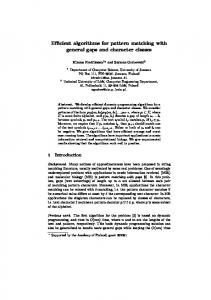
represents one complete MTP TEC. Figure 9 shows the data structure generated by SIATEC for the simple two-dimensional dataset shown in Figure 8. The data structure in Figure 9 consists of a right-directed list of three PATTERN NODEs headed by P. This list as a whole represents T 0 (D) for the dataset represented by the right-directed list headed by the global variable D. Each node in the PATTERN NODE list headed by P represents the MTP TEC E(p, D) for a single pattern in P 00 (D). For example, the first node in this list (the node pointed to by P) represents the TEC {{h1, 1i , h3, 1i} , {h1, 3i , h3, 3i}}

(29)

In this implementation, a TEC E(p, D) is represented in a compact form as an ordered pair hp, V (p, D)i where V (p, D) = {v | τ (p, v) ⊆ D} (30) In a PATTERN NODE, the pattern p is stored as a linked list headed by the pattern field and the set of vectors V (p, D) is stored as a list headed by the vectors field. Thus, the node pointed to by P in Figure 9 represents the TEC in Eq.29 by means of the ordered pair h{h1, 1i , h3, 1i} , {h0, 0i , h0, 2i}i The pattern field points to a linked list of VECTOR NODEs that represents a pattern, each VECTOR NODE storing a datapoint in the pattern. However, the datapoint associated with a VECTOR NODE in such a list is not stored explicitly as a linked list of NUMBER NODEs headed by the vector field of the node. Instead, to save space, the down field of each VECTOR NODE in a pattern list is used to point to the appropriate node in the dataset list headed by the global variable D (see Figure 9). A PATTERN NODE has both a down and a right field for the same reason that a VECTOR NODE has these fields: it allows a list of patterns to be sorted efficiently using an implementation of merge sort that converts an unsorted down-directed list into a sorted right-directed list (see the SORT PATTERN VECTOR SEQUENCES algorithm in Figure 35).

17

6 SIATEC: A CLOSER LOOK h1, 1i

h1, 3i

h3, 1i

h3, 3i

-6 -6 -6 - 6\ \ ? ? ? ? 6 6 6 2 \ -\ -\ \ \ \ ? h0, 0i \ ? h0, 2i \ \ 2 \ ?- \ -\ \ \ \ ? h0, 0i \ ? h2, 0i \ \ ? \ \ \ \ 1 \ \ -\ ? h0, 0i \ ? h0, 2i \ ? h2, 0i \ ? h2, 2i \ \ P

D

\ \

?

h2, 0i

\ \

?

h0, 2i

Figure 9: An example of a data structure generated by COMPUTE TECS.

The vec seq field in a PATTERN NODE is used to store an intervallic representation of the pattern stored in the pattern field. This intervallic representation of the pattern is used together with the cardinality of the pattern which is stored in the size field to enable a set P 00 (D) to be derived more efficiently from P (D).

6.2

Reading and preparing the dataset

Line 1 of SIATEC calls the procedure READ DATASET which is given in Figure 10. The pseudo-code used here should be easy to read for anyone who has written programs in C or Pascal using linked list data structures. If x is a pointer variable then the expression x↑y denotes the field called y in the node pointed to by x. The expression x←y should be read “x becomes equal to y”. Block structure is indicated by indentation. D, N, K, D, k and n are as defined on page 9 above. For each of the N K-dimensional datapoints p in F (the file whose name is FN—see lines 2 and 5 of READ DATASET), READ DATASET reads p, computes the required k-dimensional projection of p and stores the resulting k-dimensional datapoint in a down-directed linked list of VECTOR NODEs. This list of VECTOR NODEs is headed by the global variable D (see Figure 3). For example, if hh3, 3, 3i , h3, 3, 2i , h3, 1, 3i , h1, 1, 3i , h1, 1, 4i , h1, 3, 5ii is the sequence of 3-d datapoints stored in a file called “filename.dat” then the procedure call READ DATASET("filename.dat",110) would result in the linked list shown in Figure 11. Note that each vector in Figure 11 (and all the other data structure diagrams that follow) is actually a linked list of NUMBER NODEs but to draw these in full would clutter the diagrams. It is assumed that the function OPEN FILE (Figure 10, line 5) attempts to open the file whose name is FN returning a pointer to the beginning of the file if it succeeds and NULL if it does not. The function READ DATAPOINT (lines 8 and 12) reads the next K-dimensional datapoint from the file F returning either the required orthogonal projection of this datapoint or NULL if the end of the file has been reached. The function MAKE NEW VECTOR NODE (lines 9 and 13) simply allocates a new VECTOR NODE, initializes all its fields to NULL and returns a pointer to the new node.

18


1 2 3 4 5 6 7 8 9 10 11 12 13 14 15 16

READ DATASET(FN : dataset filename, SD : bit-vector indicating selected dimensions) local variables F : a file containing a dataset d : a pointer to a NUMBER NODE p : a VECTOR NODE pointer if (F ← OPEN FILE(FN)) = NULL EXIT D ← NULL if (d ← READ DATAPOINT(F,SD)) 6= NULL D ← MAKE NEW VECTOR NODE p ← D p↑vector ← d while (d ← READ DATAPOINT(F,SD)) 6= NULL p↑down ← MAKE NEW VECTOR NODE p ← p↑down p↑vector ← d CLOSE FILE(F)

Figure 10: READ DATASET algorithm.

D

h3, 3i h3, 1i h1, 1i h1, 1i h1, 3i h3, 3i

?\ ?\ ?\ ?\ ?\ ? \ \

Figure 11: An example linked list of VECTOR NODEs constructed by READ DATASET.

19


1 2 3 4 5 6 7 8 9 10 11 12 13 14 15 16 17 18 19 20 21 22

SORT DATASET local variables ABOVE A, A, B, BELOW B, C : VECTOR NODE pointers while D 6= NULL and D↑down 6= NULL ABOVE A ← NULL A ← D D ← NULL repeat if D 6= NULL ABOVE A↑down ← NULL B ← A↑down A↑down ← NULL BELOW B ← B↑down B↑down ← NULL C ← MERGE DATASET ROWS(A,B) if D = NULL D ← C else ABOVE A↑down ← C C↑down ← BELOW B ABOVE A ← C A ← ABOVE A↑down until A = NULL or A↑down = NULL

Figure 12: SORT DATASET algorithm. The worst-case time complexity of READ DATASET is clearly O(KN ) since it involves reading N vectors each containing K numbers. Its worst-case space complexity is O(kN ) since only k of the K numbers read from the file for each datapoint are actually stored in memory. The efficiency of this implementation of SIATEC depends upon the dataset being sorted and this sorting is done in line 2 of SIATEC using the procedure SORT DATASET shown in Figure 12. This procedure is an implementation of merge sort that converts the unsorted down-directed list generated by READ DATASET into a sorted right-directed list. On the first iteration of the outer while loop (lines 3–22), SORT DATASET scans the down-directed list of unsorted datapoints, merging each pair of consecutive datapoints into a single, sorted, right-directed list. For example, Figure 13 shows the state of the linked list D after one iteration of the outer while loop has been completed on the dataset list shown in Figure 11. On subsequent iterations, each pair of adjacent right-directed lists is merged into a single list and the process continues until the whole list has been merged into a single, sorted, right-directed list. The merging process is carried out by the algorithm MERGE DATASET ROWS shown in Figure 14. Figure 15 shows the right-directed list produced by SORT DATASET from the down-directed list shown in Figure 11. The algorithm MERGE DATASET ROWS is an implementation of the standard merge technique used in merge sort. The function VL called in lines 5 and 14 of MERGE DATASET ROWS takes two NUMBER NODE pointer arguments, each representing a vector. The procedure call VL(v 1 ,v2 ) returns TRUE if and only if v1 < v2 (vector inequality is defined in Definition 7). It is well-known that the worst-case running time for merge sort to sort a list of n items is O(n log2 n). The worst-case running time of SORT DATASET is O(kN log2 N ) where k is the dimensionality of the required orthogonal projection D of the input dataset D (see page 9) and N is the cardinality of D. This follows directly from two facts: 1) there are N items in the dataset list headed by D; and 2) each comparison carried out by VL takes O(k) time. SORT DATASET

20


D h3, 3i

?- 6\ \ h3, 3i h3, 1i

?- 6\ \ h1, 1i h1, 3i

? h1, 1i \ - 6 \ \ Figure 13: The state of the linked list D after one iteration of the outer while loop of SORT DATASET on the dataset list in Figure 11.

1 2

MERGE DATASET ROWS(A, B : VECTOR NODE pointers) local variables a, b, C, c : VECTOR NODE pointers a ← A b ← B if VL(a↑vector,b↑vector) C ← a a ← a↑right else C ← b b ← b↑right C↑right ← NULL c ← C while a 6= NULL and b 6= NULL if VL(a↑vector,b↑vector) c↑right ← a a ← a↑right else c↑right ← b b ← b↑right c ← c↑right c↑right ← NULL if a = NULL c↑right ← b else c↑right ← a return C

3 4 5 6 7 8 9 10 11 12 13 14 15 16 17 18 19 20 21 22 23 24 25 26

Figure 14: MERGE DATASET ROWS algorithm.

h1, 1i D

h1, 1i

h1, 3i

h3, 1i

h3, 3i

h3, 3i

- 6\ - 6\ - 6\ - 6\ - 6\ - 6\ \

Figure 15: The sorted, right-directed linked list produced by SORT DATASET from the unsorted, down-directed dataset list in Figure 11.

21


1 2 3 4 5 6 7 8 9 10 11 12

SETIFY DATASET local variables d1 ,d2 : VECTOR NODE pointers d1 ← D while d1 6= NULL and d1 ↑right 6= NULL if VE(d1 ↑right↑vector,d 1 ↑vector) Delete d1 ↑right. d2 ← d1 ↑right d1 ↑right ← d2 ↑right d2 ↑right ← NULL d2 ← DISPOSE OF VECTOR NODE(d 2 ) else d1 ← d1 ↑right

Figure 16: SETIFY DATASET algorithm. h1, 1i D

h1, 3i

h3, 1i

h3, 3i

- 6\ - 6\ - 6\ - 6\ \

Figure 17: The linked list that results when SETIFY DATASET has been executed on the linked list in Figure 15.

simply rearranges the nodes in the linked list created by READ DATASET and therefore uses no extra space. As explained on page 9, it is possible for more than one of the K-dimensional datapoints in D to be projected onto the same k-dimensional datapoint in D. This means that the right-directed list headed by D that results after the execution of SORT DATASET may contain duplicate datapoints. If this is so, then these datapoints will clearly be adjacent to each-other in the list and therefore can be removed using the simple procedure SETIFY DATASET shown in Figure 16. This procedure determines for each datapoint d i whether or not it is equal to the one that precedes it in the list (di−1 ) (line 5). If this is the case, then di is deleted from the list. Otherwise we proceed to comparing di+1 with di . Each datapoint in the list is therefore compared with one other preceding datapoint using the function VE which returns TRUE if and only if the two datapoints are equal. VE runs in O(k) time therefore the worst-case running time of SETIFY DATASET is O(kN ). SETIFY DATASET reduces the amount of space used by the linked list D from O(kN ) to O(kn). Figure 17 shows the linked list that results after SETIFY DATASET has been executed on the sorted right-directed dataset list shown in Figure 15.

6.3

Computing all inter-datapoint vectors

Definition 14 suggests that computing P 0 (D) would require computing the set V0 (D) = {d1 − d2 | d1 , d2 ∈ D ∧ d1 > d2 }

(31)

which is less than half the size of the set V(D) = {d1 − d2 | d1 , d2 ∈ D}

(32)

In a previous version of SIATEC, we did indeed only compute V0 (D). However, we then discovered that computing the full set V(D) allowed us to use a significantly more efficient implementation of the procedure COMPUTE TECS which is called in line 12 of SIATEC (see section 6.6 below). Indeed, by using V(D) instead

22


1 2 3 4 5 6 7 8 9 10 11 12 13 14 15 16 17 18 19 20 21 22 23 24 25

COMPUTE VECTORS local variables d1 ,d2 ,p,v : VECTOR NODE pointers V ← NULL if D 6= NULL and D↑right 6= NULL d1 ← D while d1 6= NULL p ← d1 d2 ← D while d2 6= NULL Make new VECTOR NODE under d1 . p↑down ← MAKE NEW VECTOR NODE p ← p↑down Connect p to d1 . p↑right ← d1 p↑vector ← VM(d2 ↑vector,d 1 ↑vector) if VE(d1 ↑vector,d 2 ↑vector) and d1 ↑right 6= NULL if V = NULL V ← MAKE NEW VECTOR NODE v ← V else v↑right ← MAKE NEW VECTOR NODE v ← v↑right v↑down ← p d2 ← d2 ↑right d1 ← d1 ↑right

Figure 18: COMPUTE VECTORS algorithm. of V0 (D) we were able to reduce the worst-case running time of COMPUTE TECS from O(kn 3 log2 n) in our previous version to O(kn3 ) in the version described here. In our implementation, V(D) is computed using the procedure COMPUTE VECTORS shown in Figure 18. Recall that we denote by ∆ = hδ1 , δ2 , . . . δn i the ordered set that results from sorting the dataset D = {d1 , d2 , . . . dn } so that all the datapoints are in increasing order. COMPUTE VECTORS effectively computes the table of vectors shown in Table 2. Because the dataset is sorted each row of inter-datapoint vectors in this table is sorted in increasing order from left to right and each column is sorted in increasing order from top to bottom. These two features are used to compute P 0 (D) and T 0 (D) more efficiently. In this implementation, ∆ is represented by the right-directed dataset list headed by D that results after SETIFY DATASET has been executed in line 3 of SIATEC (see Figure 19). Figure 20 shows the structure computed by COMPUTE VECTORS for the dataset list shown in Figure 19. This data structure is essentially a linked list representation of Table 2. Let us denote by Φv the VECTOR NODE in the structure in Figure 20

δ1

D

δ2

- 6\ - 6\

δn

- 6\ \

Figure 19: The linked list representation of the sorted dataset ∆.

23


To

δ1

δ2

From ···

δn−1

δn

δ1 δ2 .. .

δ1 − δ 1 δ2 − δ 1 .. .

δ1 − δ 2 δ2 − δ 2 .. .

··· ··· .. .

δ1 − δn−1 δ2 − δn−1 .. .

δ1 − δ n δ2 − δ n .. .

δn−1 δn

δn−1 − δ1 δn − δ 1

δn−1 − δ2 δn − δ 2

··· ···

δn−1 − δn−1 δn − δn−1

δn−1 − δn δn − δ n

Table 2: The table of vectors represented by the data structure generated by COMPUTE VECTORS. δ1

D - 6 ?6 δ1 -δ1 ? δ2 -δ1 6 6

V

-\

δ2

δn−1

-6 -6 ? 6 δ1 -δn-1 ?6 δ1 -δ2 ? ? δ2 -δ2 6 δ2 -δn-1 6 6 ? 6 δ -δ ? 6δ -δ ? 6 δn-1 -δ1 n-1 n-1 n-1 2 6 ? 6 δ -δ \? ? δn -δ1 \ 6 n 2 6 δn -δn-1 6\ 6 -\ - \ 6\

δn

- 6\ ?6 δ1 -δn ? δ2 -δn 6 ? 6 ? δn -δn \ 6

δn-1 -δn

Figure 20: The data structure generated by COMPUTE VECTORS.

whose vector field stores the result of evaluating a sentence denoted by v. COMPUTE VECTORS constructs for each datapoint node Φδi a down-directed list of VECTOR NODEs, Φδ1 −δi down to Φδn −δi , headed by Φδi ↑down (see Figure 20). Note that Φδj −δi ↑right = Φδi for each node Φδj −δi . Note also that COMPUTE VECTORS constructs the right-directed linked list V which stores the node Φδi −δi for each datapoint δi . These two features are used to compute the set P 0 (D) more efficiently (see section 6.4 below). COMPUTE VECTORS calculates the vector d1 − d2 for all pairs of datapoints d1 , d2 ∈ D, making a total of n2 vectors to be computed. Each of these vector subtractions is carried out by the function VM called in line 15. This function takes two NUMBER NODE pointer arguments, each representing a vector. The call VM(v1,v2 ) returns a pointer to a NUMBER NODE list representing the vector v 1 − v2 . Each of these n2 vector subtractions takes O(k) time (recall that k is the dimensionality of D, the required orthogonal projection of D). This implies that the worst-case running time of COMPUTE VECTORS is O(kn 2 ). The resulting data structure, as can be seen in Figure 20, occupies O(kn2 ) space.

6.4

Computing P 0 (D)

Lines 5 to 7 of SIATEC compute the set P 0 (D) defined in Eq.13 above. The fact that Φδj −δi ↑right = Φδi

24


1 2

CONSTRUCT VECTOR TABLE local variables p, v, w : VECTOR NODE pointers p ← V while p 6= NULL v ← p↑down↑down w ← p while v 6= NULL w↑down ← MAKE NEW VECTOR NODE w ← w↑down w↑right ← v v ← v↑down p ← p↑right

3 4 5 6 7 8 9 10 11 12

Figure 21: CONSTRUCT VECTOR TABLE algorithm. V

-\ \ \ \

\ \

?-Φ δ2 −δ1 ?-Φ δ3 −δ1 ?-Φ

-\

δ4 −δ1

?-Φδ −δ 1 n−1 ? Φ \ δn −δ1

\ \

\ \

-\ ?-Φ δ3 −δ2 ?-Φ δ4 −δ2

?-Φδ −δ 2 n−1 ? \ -Φ δn −δ2

\

\ \

-\

\

?-Φ δ4 −δ3 ?-Φδ −δ 3 n−1 ? \ -Φ δn −δ3

?-Φδ −δ n n−1

\ \

Figure 22: The data structure V constructed by CONSTRUCT VECTOR TABLE.

in the data structure shown in Figure 20 means that P 0 (D) can be computed simply by sorting the nodes corresponding to the vectors below the leading diagonal of Table 2.2 However, the efficient computation of T 0 (D) carried out by COMPUTE TECS in line 12 of SIATEC relies upon the fact that the down-directed VECTOR NODE lists (Φδ1 −δi to Φδn −δi in Figure 20) remain sorted in increasing order from top to bottom. Therefore we cannot actually change the order of the nodes in Figure 20. To get around this problem, we use the linked list V in Figure 20 and the procedure CONSTRUCT VECTOR TABLE (Figure 21) to construct the data structure shown in Figure 22. This data structure is a representation of the region of Table 2 below the leading diagonal and the nodes in this data structure can safely be sorted without disturbing the arrangement in Figure 20. The data structure in Figure 22 consists of n − 1 down-directed lists. The list headed by the down node of the jth node in the right-directed list headed by V contains n − j nodes. There are therefore n(n−1) 2 nodes constructed by CONSTRUCT VECTOR TABLE. The worst-case running time of CONSTRUCT VECTOR TABLE is therefore O(n2 ) (note that this is independent of k, the dimensionality of D). The total space used by SIATEC up to the completion of CONSTRUCT VECTOR TABLE remains O(kn 2 ). We shall now present an example of how simply sorting the data structure in Figure 22 yields P 0 (D). Let us consider the dataset in Figure 23. Figure 24 shows the table of vectors represented by the data structure V computed by CONSTRUCT VECTOR TABLE for this dataset. This table corresponds to the data 2 If we denote by v i,j the location in the ith column and jth row of a matrix or table (counting left-to-right and top-tobottom respectively), then the leading diagonal is the set of locations {v i,j | i = j}.

25


×

3

× ×

2 y ×

1

×

×

0 0

1

x

2

3

Figure 23: A simple two-dimensional dataset.

From h1, 1i

6

h1, 3i

6

h2, 1i

6

h2, 2i

6

h1, 3i

h0, 2i

h2, 1i

h1, 0i

h1, −2i

To h2, 2i

h1, 1i

h1, −1i

h0, 1i

h2, 3i

h1, 2i

h1, 0i

h0, 2i

h0, 1i

h3, 2i

h2, 1i

h2, −1i

h1, 1i

h1, 0i

h2, 3i

6

h1, −1i

Figure 24: The vector table constructed by CONSTRUCT VECTOR TABLE for the dataset in Figure 23.

26


Datapoint

Vector h0, 1i h0, 1i h0, 2i h0, 2i h1, −2i h1, −1i h1, −1i h1, 0i h1, 0i h1, 0i h1, 1i h1, 1i h1, 2i h2, −1i h2, 1i

-

h2, 1i h2, 2i h1, 1i h2, 1i h1, 3i h1, 3i h2, 3i h1, 1i h1, 3i h2, 2i h1, 1i h2, 1i h1, 1i h1, 3i h1, 1i

Figure 25: The list that results from sorting the vectors in the table in Figure 24.

structure shown in Figure 22. Each entry in the table in Figure 24 is linked to the datapoint at the top of its column to represent the fact that Φδj −δi ↑right = Φδi in Figure 20. We now sort the entries in the table in Figure 24 to obtain the list of vectors shown in Figure 25. Note that each vector v in this list is still linked to the datapoint at the head of the column in Figure 24 that contained v. Simply reading off all the datapoints attached to the adjacent occurrences of a given vector v in this list yields the maximal translatable pattern for v. P 0 (D) can be obtained simply by scanning the list once, reading off the attached datapoints and starting a new pattern each time the vector changes. Each box in the right-hand column of Figure 25 corresponds to a maximal translatable pattern. From the foregoing discussion, it should be clear that the next step after executing CONSTRUCT VECTOR TABLE is to sort the nodes in the resulting data structure (Figure 22). This is done using SORT VECTORS (Figure 26), an implementation of merge sort that converts the structure in Figure 22 into a single, sorted, down-directed list representing a list of vectors like the one in Figure 25. SORT VECTORS works in a way that is essentially identical to SORT DATASET (see Figure 12). Each pair of adjacent down-directed lists in Figure 22 is merged into a single list using the procedure MERGE VECTOR COLUMNS (Figure 27) which is called in line 14 of SORT VECTORS. Each iteration of the main while loop (Figure 26, lines 3 to 22) corresponds to one pass along the right-directed list of lists headed by V. This while loop terminates when the complete structure has been converted into a single down-directed list—that is, when V↑right = NULL. This leaves a single sentinel node at the top of the list that is not associated with any vector. This sentinel is removed in lines 23 to 28 of SORT VECTORS producing a sorted, down-directed list like the one in Figure 28. The procedure DISPOSE OF VECTOR NODE called in line 27 of SORT VECTORS takes a single VECTOR NODE pointer argument v. It deallocates the VECTOR NODE pointed to by v and any other nodes connected to v. Therefore, if one wishes to remove only the node

27


1 2 3 4 5 6 7 8 9 10 11 12 13 14 15 16 17 18 19 20 21 22 23 24 25 26 27 28

SORT VECTORS local variables BEFORE A, A, B, AFTER B, C : VECTOR NODE pointers while V 6= NULL and V↑right 6= NULL BEFORE A ← NULL A ← V V ← NULL repeat if V 6= NULL BEFORE A↑right ← NULL B ← A↑right A↑right ← NULL AFTER B ← B↑right B↑right ← NULL C ← MERGE VECTOR COLUMNS(A,B) if V = NULL V ← C else BEFORE A↑right ← C C↑right ← AFTER B BEFORE A ← C A ← BEFORE A↑right until A = NULL or A↑right = NULL Finally we delete the sentinel node pointed to by V. if V 6= NULL A ← V↑down V↑down ← NULL DISPOSE OF VECTOR NODE(V) V ← A

Figure 26: SORT VECTORS algorithm.

28


1 2

MERGE VECTOR COLUMNS(A, B : VECTOR NODE pointers) local variables a, b, C, c : VECTOR NODE pointers

3 4 5 6 7 8 9 10 11 12 13 14 15 16 17 18 19 20 21

a ← A↑down b ← B↑down C ← A C↑down ← NULL c ← C while a 6= NULL and b 6= NULL if VL(b↑right↑vector,a↑right↑vector) c↑down ← b b ← b↑down else c↑down ← a a ← a↑down c ← c↑down c↑down ← NULL if a = NULL c↑down ← b else c↑down ← a return C

Figure 27: MERGE VECTOR COLUMNS algorithm. pointed to by v, both the down and right fields of v should be NULL before DISPOSE OF VECTOR NODE is called. The number of items to be sorted by SORT VECTORS is equal to n(n−1) , the number of entries below 2 the leading diagonal in Table 2. Each comparison involves a call to VL in line 9 of MERGE VECTOR COLUMNS which takes O(k) time. The worst-case running time of SORT VECTORS is therefore O(kn 2 log2 (n2 )) = O(kn2 log2 n). No extra space is used in the process. In fact, the total amount of spaced used is reduced by n−1 VECTOR NODEs because each sentinel node that heads a down-directed list in Figure 22 is removed. The total worst-case space used by SIATEC up to the completion of SORT VECTORS therefore remains O(kn 2 ). We now present a formal proof that SORT VECTORS yields P 0 (D). The data structure generated by CONSTRUCT VECTOR TABLE (see Figures 22 and 24) is essentially a representation of the set of ordered pairs Z(D), defined as follows. Definition 16 If D is a dataset then Z(D) = {hd2 − d1 , d1 i | d1 , d2 ∈ D ∧ d2 > d1 }

(33)

We now prove two lemmas concerning Z(D). Lemma 7 If D is a dataset and d1 , d2 , d3 , d4 ∈ D then d2 6= d4 ∨ d1 6= d3 ⇒ hd1 − d2 , d2 i 6= hd3 − d4 , d4 i Proof

(34)

29


h1, 1i D V h0, 1i

\

?- 6

\

?- 6

\

?- 6

\

?- 6

\

?- 6

\

?- 6

\

?- 6

\

?- 6

\

?- 6

\

?- 6

\

?- 6

\

?- 6

\

?- 6

\

?- 6

h1, 3i

h2, 1i

h2, 2i

h2, 3i

h3, 2i

- 6 - 6 - 6 - 6 - 6 - 6\ \ 6 6 6 6 6

h0, 1i

h0, 2i

h0, 2i

h1, −2i

h1, −1i

h1, −1i

h1, 0i

h1, 0i

h1, 0i

h1, 1i

h1, 1i

h1, 2i

h2, −1i

h2, 1i

?- 6

\ \

Figure 28: The data structure headed by V at the conclusion of SORT VECTORS for the dataset in Figure 23.

30


d2 6= d4 d1 6= d3 ∧ d2 = d4

⇒

hd1 − d2 , d2 i 6= hd3 − d4 , d4 i

⇒

d1 − d2 6= d3 − d4

⇒

hd1 − d2 , d2 i 6= hd3 − d4 , d4 i

(35) (36)

Eq.35 and Eq.36 together imply that d2 6= d4 ∨ d1 6= d3 ⇒ hd1 − d2 , d2 i 6= hd3 − d4 , d4 i

Lemma 8 If D is a dataset of order n then |Z(D)| =

n(n − 1) 2

(37)

Proof Definition 16 and Lemma 7 together imply that |Z(D)| is equal to the number of elements in the set {hd1 , d2 i | d1 , d2 ∈ D ∧ d2 > d1 }

(38)

which has the same cardinality as the set {{d1 , d2 } | d1 , d2 ∈ D}

(39)

The cardinality of the set in Eq.39 is equal to the number of distinct combinations possible when 2 distinct objects are drawn from a set of n distinct objects. This implies that ! n |Z(D)| = 2 = =

n! (n − 2)!2! n(n − 1) 2

Definition 17 If D is a dataset and z is an ordered pair of the form he − d, di where e, d ∈ D then F (z, Z(D)) = {y | y ∈ Z(D) ∧ y[1] = z[1]}

(40)

Figure 25 shows the complete set Z(D) for the dataset in Figure 23. Each row in this list corresponds to an ordered pair z = hd2 − d1 , d1 i in Z(D). By sorting Z(D) so that the vectors are in increasing order, the list has effectively been partitioned into classes of adjacent rows such that each class contains all the ordered pairs z for a particular vector. Each of these classes of ordered pairs corresponds to a set F (z, Z(D)). For example, if we denote the dataset in Figure 23 by D1 , then the first class of ordered pairs in the list in Figure 25 corresponds to the set F (hh0, 1i , h2, 1ii , Z(D1 )) = {hh0, 1i , h2, 1ii , hh0, 1i , h2, 2ii}

31


Definition 18 If D is a dataset then Z(D) = {F (z, Z(D)) | z ∈ Z(D)}

(41)

The set Z(D) corresponds to the partition of Z(D) represented by the sorted list that results after SORT VECTORS has been executed (see Figures 25 and 28). We now prove formally that Z(D) is indeed a partition of Z(D). Lemma 9 If D is a dataset then Z(D) is a partition of Z(D). Proof To prove this lemma, we need to prove all three of the following: z ∈ Z(D) ⇒ (∃F | F ∈ Z(D) ∧ z ∈ F )

(42)

F ∈ Z(D) ∧ z ∈ F ⇒ z ∈ Z(D)

(43)

F1 , F2 ∈ Z(D) ∧ F1 6= F2 ∧ z ∈ F1 ⇒ z ∈ / F2

(44)

From Definition 17 we know that z ∈ Z(D) ∧ z[1] = z[1] ⇒ z ∈ F (z, Z(D)) Clearly z[1] = z[1] therefore z ∈ Z(D) ⇒ z ∈ F (z, Z(D))

(45)

z ∈ Z(D) ⇒ F (z, Z(D)) ∈ Z(D)

(46)

From Definition 18 we know that Eq.45 and Eq.46 together prove Eq.42. From Definition 18 we can deduce that F ∈ Z(D) ⇒ ∃y | F = F (y, Z(D)) ∧ y ∈ Z(D)

(47)

Let y ∈ Z(D) and let F = F (y, Z(D)). If F = F (y, Z(D)) ∧ y ∈ Z(D) ∧ z ∈ F then it follows that z ∈ F (y, Z(D)) ∧ y ∈ Z(D)

(48)

But from Definition 17 we know that if Eq.48 holds then z ∈ Z(D) which proves Eq.43. From Definition 18 we know that F1 ∈ Z(D)

⇒

∃z1 | F1 = F (z1 , Z(D)) ∧ z1 ∈ Z(D)

(49)

F2 ∈ Z(D)

⇒

∃z2 | F2 = F (z2 , Z(D)) ∧ z2 ∈ Z(D)

(50)

Let z1 , z2 ∈ Z(D) and let F1 = F (z1 , Z(D)) and F2 = F (z2 , Z(D)). It follows from Definition 17 that F1 6= F2

⇒

F (z1 , Z(D)) 6= F (z2 , Z(D))

⇒

{y | y ∈ Z(D) ∧ y[1] = z1 [1]} 6= y 0 | y 0 ∈ Z(D) ∧ y 0 [1] = z2 [1]

⇒

(∃y 0 | y 0 [1] = z2 [1] ∧ y 0 [1] 6= z1 [1]) ∨ (∃y | y[1] = z1 [1] ∧ y[1] 6= z2 [1])

⇒

z2 [1] 6= z1 [1]

(51)

From Definition 17 it follows directly that z ∈ F1 ⇒ z ∈ Z(D) ∧ z[1] = z1 [1] From Eq.51 and Eq.52 we deduce that z ∈ F1 ⇒ z[1] 6= z2 [1]

(52)

32


which, taken with Definition 17, implies z∈ / F (z2 , Z(D)) ⇒ z ∈ / F2 thus proving Eq.44.

We now prove that the number of nodes in the down-directed list generated by SORT VECTORS is always n(n−1) . 2

Lemma 10 If D is a dataset then X

F ∈Z(D)

|F | =

n(n − 1) 2

(53)

Proof From Lemma 9 we know that Z(D) is a partition of Z(D). Therefore X |F | = |Z(D)| F ∈Z(D)

But from Lemma 8 we know that |Z(D)| =

n(n − 1) 2

therefore X

|F | =

F ∈Z(D)

n(n − 1) 2

Definition 19 If F ∈ Z(D) then

π(F ) = {y[2] | y ∈ F }

Each boxed set of datapoints in the right-hand column of Figure 25 corresponds to π(F (z, Z(D))) for one of the classes F (z, Z(D)) ∈ Z(D). (Recall that the sorted list in Figure 25 represents the partition Z(D) for the dataset in Figure 23). Lemma 11 If D is a dataset and z ∈ Z(D) then |π(F (z, Z(D)))| = |F (z, Z(D))|

(54)

Proof From Definition 17 it follows that if z1 , z2 ∈ F (z, Z(D)) then z1 [1] = z2 [1]. This, in turn, implies that if z1 , z2 ∈ F (z, Z(D)) and z1 6= z2 then z1 [2] 6= z2 [2]. This, together with Definition 19 implies that |π(F (z, Z(D)))| = |F (z, Z(D))|.

We now prove that each of the boxed sets of datapoints in Figure 25 is the maximal translatable pattern for the vector associated with it. Theorem 1 If D is a dataset and z ∈ Z(D) then π(F (z, Z(D))) = p(z[1], D)

(55)

33


Proof Definition 11 implies that p(z[1], D) = {d | d ∈ D ∧ d + z[1] ∈ D}

(56)

π(F (z, Z(D))) = {y[2] | y ∈ F (z, Z(D))}

(57)

Definition 19 implies that Definition 17 and Eq.57 imply that π(F (z, Z(D)))

=

{y[2] | y ∈ {x | x ∈ Z(D) ∧ x[1] = z[1]}}

=

{y[2] | y ∈ Z(D) ∧ y[1] = z[1]}

(58)

Eq.58 and Definition 16 imply π(F (z, Z(D)))

=

{y[2] | y ∈ {hd2 − d1 , d1 i | d1 , d2 ∈ D ∧ d2 > d1 } ∧ y[1] = z[1]}

=

{d1 | d1 , d2 ∈ D ∧ d2 > d1 ∧ z[1] = d2 − d1 }

=

{d1 | d1 , d2 ∈ D ∧ d2 > d1 ∧ d2 = d1 + z[1]}

(59)

It is clear that d2 > d1 ∧ d2 = d1 + z[1] ⇐⇒ z[1] > 0 ∧ d2 = d1 + z[1]

(60)

Eq.59 and Eq.60 together imply π(F (z, Z(D))) = {d1 | d1 , d2 ∈ D ∧ z[1] > 0 ∧ d2 = d1 + z[1]}

(61)

z ∈ Z(D) ⇒ z[1] > 0

(62)

Definition 16 implies that Eq.61 and Eq.62 imply π(F (z, Z(D)))

=

{d1 | d1 , d2 ∈ D ∧ d2 = d1 + z[1]}

=

{d1 | d1 ∈ D ∧ d1 + z[1] ∈ D}

(63)

Eq.56 and Eq.63 imply π(F (z, Z(D))) = p(z[1], D)

Definition 20 If D is a dataset then Π(D) = {π(F (z, Z(D))) | z ∈ Z(D)}

(64)

If D1 is the dataset in Figure 23 then Π(D1 ) is the set that only contains every boxed set of datapoints in the right-hand column of Figure 25. We now prove that Π(D) = P 0 (D) and therefore that the sorted list of nodes generated by SORT VECTORS does indeed represent P 0 (D). Theorem 2 If D is a dataset then P 0 (D) = Π(D)

(65)

Π(D) = {p(z[1], D) | z ∈ Z(D)}

(66)

Proof Theorem 1 and Definition 20 imply

34


Eq.66 and Definition 16 imply Π(D)

=

{p(z[1], D) | z ∈ {hd2 − d1 , d1 i | d1 , d2 ∈ D ∧ d2 > d1 }}

=

{p(d2 − d1 , D) | d1 , d2 ∈ D ∧ d2 > d1 }

(67)

Eq.67 and Definition 14 imply P 0 (D) = Π(D)

We now prove that the sum of the sizes of all the maximal translatable patterns in P 0 (D) is less than . or equal to n(n−1) 2 Theorem 3 If D is a dataset of cardinality n then X

|p| ≤

X

|p| =

p∈P 0 (D)

n(n − 1) 2

(68)

Proof Theorem 2 implies that X

p∈P 0 (D)

Defs.18, 19 and 20 imply

|π|

(69)

π∈Π(D)

|Π(D)| ≤ |Z(D)| Lemma 11, Eq.70, Definition 18 and Definition 20 taken together imply X X |π| ≤ |F |

(70)

(71)

F ∈Z(D)

π∈Π(D)

Eq.71 and Lemma 10 imply that X

|π| ≤

n(n − 1) 2

X

|p| ≤

n(n − 1) 2

π∈Π(D)

Eq.72 and Eq.69 imply

p∈P 0 (D)

(72)

Theorem 3 follows from the fact that Π(D) is derived from Z(D) simply by partitioning Z(D). Theorem 3 is critical for computing the worst-case running time of the procedures called in lines 7 to 13 of SIATEC. As explained above, the data structure generated by SORT VECTORS can be used directly to output P 0 (D). However, the purpose of SIATEC is to compute T 0 (D) and this process can be simplified by converting the data structure produced by SORT VECTORS (Figures 25 and 28) into a more explicit representation of P 0 (D). This conversion is carried out using the procedure CONSTRUCT PATTERN LIST defined in Figure 29. CONSTRUCT PATTERN LIST is called in line 7 of SIATEC. Figure 30 shows the data structure that results when CONSTRUCT PATTERN LIST is carried out on the data structure shown in Figure 28. As can be seen in Figure 30, CONSTRUCT PATTERN LIST builds a down-directed list of PATTERN NODEs. The pattern field of each of these nodes is made to point to a right-directed list of VECTOR NODEs that indirectly represents one of the maximal translatable patterns in P 0 (D). The function MAKE NEW PATTERN NODE called in line 7 of CONSTRUCT PATTERN LIST allocates a new PATTERN NODE, setting its size field to 0 and all its pointer fields to NULL.

35


1 2 3 4 5 6 7 8 9 10 11 12 13 14 15 16 17 18 19 20 21 22

CONSTRUCT PATTERN LIST local variables p : a PATTERN NODE pointer v1 , v2 , q : VECTOR NODE pointers P ← NULL if V 6= NULL v1 ← V P ← MAKE NEW PATTERN NODE p ← P while v1 6= NULL p↑pattern ← MAKE NEW VECTOR NODE q ← p↑pattern q↑down ← v1 ↑right↑right v2 ← v1 ↑down while v2 6= NULL and VE(v2 ↑right↑vector,v 1 ↑right↑vector) q↑right ← MAKE NEW VECTOR NODE q ← q↑right q↑down ← v2 ↑right↑right v2 ← v2 ↑down v 1 ← v2 if v1 6= NULL p↑down ← MAKE NEW PATTERN NODE p ← p↑down

Figure 29: CONSTRUCT PATTERN LIST algorithm.

h1, 1i

\ \ 0 \ \ 0 \ \ 0 \ \ 0 \ \ 0 \ \ 0 \ \ 0 \ \ 0 \ \ 0

h1, 3i

h2, 1i

h2, 2i

h2, 3i

h3, 2i

\ \ D - 6 - 6 - 6 - 6 - 6 - 6 P 6 6 6 6 6 ?\ -\ -\ \ ?\ - \ -\ \ ?\ -\ \ ?\ -\ -\ \ ?\ - \ - \ -\ \ ?\ - \ -\ \ ?\ - \ \ ?\ -\ \ ? \ \ -\ \

Figure 30: The data structure that results after CONSTRUCT PATTERN LIST has executed for the dataset in Figure 23.

36


1 2 3 4 5 6 7 8 9 10 11 12 13 14

VECTORIZE PATTERNS local variables p : a PATTERN NODE pointer v, q : VECTOR NODE pointers p ← P while p 6= NULL p↑vec seq ← MAKE NEW VECTOR NODE v ← p↑vec seq q ← p↑pattern while q↑right 6= NULL v↑right ← MAKE NEW VECTOR NODE v ← v↑right v↑vector ← VM(q↑right↑down↑vector,q↑down↑vector) q ← q↑right p ← p↑down

Figure 31: VECTORIZE PATTERNS algorithm. CONSTRUCT PATTERN LIST simply scans once the down-directed list headed by V (see Figure 28). For each node, if the vector is different from the last one a new PATTERN NODE is created and if the vector is the same as the last one a new VECTOR NODE is added to the pattern list for the current PATTERN NODE. The worst-case running time of CONSTRUCT PATTERN LIST is proportional to the length of the list headed by V which was shown above to be n(n−1) (Lemma 8). The running time is therefore O(kn2 ) because for 2 each node in the list, the function VE (whose running time is O(k)) must be executed (Figure 29, line 14). After execution of CONSTRUCT PATTERN LIST the overall space complexity of SIATEC remains O(kn 2 ).

6.5

Computing P 00 (D)

An examination of Figure 30 reveals that the pattern {h1, 1i , h2, 1i} occurs twice—it is the maximal translatable pattern for both the vector h0, 2i and the vector h1, 1i (see Figure 25). It can also be seen that another pattern in the list is {h1, 3i h2, 3i} which is translationally equivalent to {h1, 1i , h2, 1i}. Clearly, all these patterns are members of the same TEC so we only need to compute the TEC of one of these patterns. Therefore, as described on page 13, before computing T 0 (D) we compute the partition P(D) (defined in Eqs.26 and 27) and then construct a set P 00 (D) that contains exactly one pattern from each E ∈ P(D). This guarantees that there are no patterns in P 00 (D) that are translationally equivalent, thus ensuring that the procedure COMPUTE TECS (Figure 2, line 12) does no more work than necessary. The procedures called in lines 8 to 11 of SIATEC construct such a set P 00 (D) from the list of patterns generated by CONSTRUCT PATTERN LIST. The first step in this process is carried out by the procedure VECTORIZE PATTERNS which is called in line 8 of SIATEC. This procedure is defined in Figure 31. For each pattern p in the list headed by the global variable P that results after the execution of CONSTRUCT PATTERN LIST (see Figure 30), VECTORIZE PATTERNS computes an intervallic representation of p which is stored in the vec seq field of the PATTERN NODE representing p. Figure 32 shows the data structure that results when VECTORIZE PATTERNS has been executed on the data structure shown in Figure 30. Each pattern is represented in the data structure as a right-directed list headed by the pattern field of a PATTERN NODE. This right-directed list actually represents an ordered set of datapoints in which the datapoints are in increasing order. This ordering is a result of the way that SORT VECTORS operates and the

37


h1, 1i D

h1, 3i

h2, 1i

h2, 2i

h2, 3i

h3, 2i

- 6 - 6 - 6 - 6 - 6 - 6\ \ 6 6 6 6 6

P

h0, 1i

\?\

\ \

\ 0

?\

-\

h1, 0i

\?\

\ \

\ 0

?\ - \

-\

\ \ \

\ 0

?\

-\

\ \

\ 0

?\

-\

6\?

\ \

\ 0

?\ - \

-\

\?\

\ \

\ 0

?\ - \

\ \ \

\ 0

?\ - \

\ \ \

\ 0

?\

\ \ \

\ 0 \ \

h1, 0i h1, −1i

6\ \ 6 h1, 0i

\?\ h0, 2i

? -\

-\

\

\

\

-\ -\ -\

\

\

\

\

-\

\

\

Figure 32: The data structure that results after VECTORIZE PATTERNS has executed for the dataset in Figure 23.

38


fact that the dataset list is sorted. The fact that each pattern representation is ordered in this way means that two patterns will have an identical intervallic representation as computed by VECTORIZE PATTERNS if and only if they are translationally equivalent (see, for example, the second, fourth and sixth patterns in the list shown in Figure 32). We now formalize this concept of “intervallic representation”. Definition 21 An object β is a vector sequence if and only if it is an ordered set of vectors. β is a k-dimensional vector sequence if and only if every vector in β has cardinality k. Let pi = di,1 , di,2 , . . . di,|pi | be one of the patterns in the list of patterns generated by CONSTRUCT PATTERN LIST and let γi = δi,1 , δi,2 , . . . δi,|pi | be the ordered set of datapoints that results from sorting pi so that the datapoints are in increasing order. The procedure VECTORIZE PATTERNS takes each pattern p i and computes the vector sequence |pi |−1

βi =

M j=1

hδi,j+1 − δi,j i

(73)

The worst-case running time of VECTORIZE PATTERNS is linear in the sum of the cardinalities of all the patterns pi which was shown in Lemma 10 to be equal to n(n − 1) 2 For each datapoint but one in each pattern, the vector subtraction in line 12 of VECTORIZE PATTERNS must be computed. Each of these vector subtractions takes O(k) time therefore the overall worst-case running time of VECTORIZE PATTERNS is O(kn2 ). The overall space used remains O(kn2 ). If the PATTERN NODEs headed by P are sorted by their vec seq fields then all the patterns with a given intervallic representation will be adjacent to each-other in the list and we will effectively have computed the partition P(D). Clearly, if two patterns have different cardinalities then they are not translationally equivalent. We can therefore make this sorting process more efficient by first computing the cardinality of each pattern and storing this integer in the size field of the PATTERN NODE for the pattern. This is more efficient than computing the pattern cardinalities “on the fly” during the sorting process itself. Using the latter strategy, each time a pair of patterns is compared one must compute the cardinalities of both patterns. If there are m patterns, then using merge sort this would involve O(m log 2 m) pattern-cardinality computations whereas if we simply compute the cardinalities of the patterns in advance, only O(m) pattern-cardinality computations are necessary. This one-time computation of pattern cardinalities is carried out by the procedure COMPUTE PATTERN SIZES which is defined in Figure 33. The worst-case running time for COMPUTE PATTERN SIZES is proportional to the sum of the cardinalities of the patterns in the list headed by P. From Lemma 10 we can deduce that this running time is therefore O(n2 ). This running time is independent of the dimensionality of the dataset since we are simply counting the number of datapoints in each pattern. Figure 34 shows the data structure that results after COMPUTE PATTERN SIZES has been executed for the dataset in Figure 23. The only difference between Figure 34 and Figure 32 is that each pattern’s cardinality has been computed and stored in the size field of the pattern’s PATTERN NODE.

39


1 2 3

COMPUTE PATTERN SIZES local variables p : a PATTERN NODE pointer q : a VECTOR NODE pointer p ← P while p 6= NULL q ← p↑pattern p↑size ← 0 while q 6= NULL p↑size ← p↑size + 1 q ← q↑right p ← p↑down

4 5 6 7 8 9 10 11

Figure 33: COMPUTE PATTERN SIZES algorithm.

h1, 1i D

h1, 3i

h2, 1i

h2, 2i

h2, 3i

h3, 2i

- 6 - 6 - 6 - 6 - 6 - 6\ \ 6 6 6 6 6

P

h0, 1i

\?\

\ \

\ 2

?\

-\

h1, 0i

\?\

\ \

\ 2

?\ - \

-\

\ \ \

\ 1

?\

-\

\ \

\ 2

?\

-\

6\?

\ \

\ 3

?\ - \

-\

\?\

\ \

\ 2

?\ - \

\ \ \

\ 1

?\ - \

\ \ \

\ 1

?\

\ \ \

\ 1 \ \

h1, 0i h1, −1i

6\ \ 6 h1, 0i

\?\ h0, 2i

? -\

-\

\

\

\

-\ -\ -\

\

\

\

\

-\

\

\

Figure 34: The data structure that results after COMPUTE PATTERN SIZES has executed for the dataset in Figure 23.

40


1 2 3 4 5 6 7 8 9 10 11 12 13 14 15 16 17 18 19 20 21 22

SORT PATTERN VECTOR SEQUENCES local variables ABOVE A, A, B, BELOW B, C : PATTERN NODE pointers while P 6= NULL and P↑down 6= NULL ABOVE A ← NULL A ← P P ← NULL repeat if P 6= NULL ABOVE A↑down ← NULL B ← A↑down A↑down ← NULL BELOW B ← B↑down B↑down ← NULL C ← MERGE PATTERN ROWS(A,B) if P = NULL P ← C else ABOVE A↑down ← C C↑down ← BELOW B ABOVE A ← C A ← ABOVE A↑down until A = NULL or A↑down = NULL

Figure 35: SORT PATTERN VECTOR SEQUENCES algorithm. The partition P(D) can now be computed efficiently by simply sorting the down-directed list of PATTERN NODEs headed by P. This is done using the procedure SORT PATTERN VECTOR SEQUENCES (Figure 35), an implementation of merge sort that converts the unsorted down-directed list headed by P into a sorted right-directed list. SORT PATTERN VECTOR SEQUENCES works in essentially the same way as SORT DATASET (Figure 12). The function MERGE PATTERN ROWS called in line 14 of SORT PATTERN VECTOR SEQUENCES merges two sorted right-directed lists into a single list using the comparison function PVSL. MERGE PATTERN ROWS is defined in Figure 36 and PVSL is defined in Figure 37. We now formalize the concept of vector sequence inequality that is used in SORT PATTERN VECTOR SEQUENCES. Definition 22 If β1 and β2 are two vector sequences then β1 < β 2 if and only if one of the following conditions is satisfied: 1. |β1 | < |β2 |; 2. |β1 | = |β2 | and β1 [1] < β2 [1]; 3. |β1 | = |β2 | and there exists an integer j such that j > 1 and β1 [j] < β2 [j] and β1 [i] = β2 [i] for all i such that 1 ≤ i < j.

41


1 2 3 4 5 6 7 8 9 10 11 12 13 14 15 16 17 18 19 20 21 22 23 24 25 26

MERGE PATTERN ROWS(A, B : PATTERN NODE pointers) local variables a, b, C, c : PATTERN NODE pointers a ← A b ← B if PVSL(b,a) C ← a a ← a↑right else C ← b b ← b↑right C↑right ← NULL c ← C while a 6= NULL and b 6= NULL if PVSL(b,a) c↑right ← a a ← a↑right else c↑right ← b b ← b↑right c ← c↑right c↑right ← NULL if a = NULL c↑right ← b else c↑right ← a return C

Figure 36: MERGE PATTERN ROWS algorithm.

1 2 3 4 5

PVSL(p 1 , p2 : PATTERN NODE pointers) if p1 ↑size < p2 ↑size return TRUE if p1 ↑size > p2 ↑size return FALSE return VEC LIST LESS THAN(p 1 ↑vec seq↑right, p2 ↑vec seq↑right)

Figure 37: PVSL algorithm.

42


1 2 3 4 5 6 7

VEC LIST LESS THAN(p1 , p2 : VECTOR NODE pointers) if p1 = NULL and p2 = NULL return FALSE if VL(p1 ↑vector, p2 ↑vector) return TRUE if VL(p2 ↑vector, p1 ↑vector) return FALSE return VEC LIST LESS THAN(p 1 ↑right, p2 ↑right)

Figure 38: VEC LIST LESS THAN algorithm. The function PVSL implements the binary relation ‘ βy+1 we compare β2 with βy+1 and append the greater of the two to C. This continues until either all the elements of A or all the elements of B have

44


been appended to C at which point all the remaining unmerged elements are appended to C in a single step to give the desired result. As can be seen, this process involves carrying out a series of comparisons in which an element of A is compared with an element of B to determine which of the two is the greater. Each of these comparisons results in a new element being appended to C. In the worst case, the number of comparisons to be carried out is |A| + |B| − 1. It is clear from Definition 22 that the worst-case running time for comparing two k-dimensional vector sequences, β1 and β2 , is ck |βmin | where c is a constant and βmin is the lesser of β1 and β2 . For each element βi in A or B, we know that βi is the greater vector sequence in at most one comparison because if βi is the greater sequence in a comparison it is immediately appended to C and is not compared with any other member of A or B after that. We therefore know that the time taken to carry out the comparison that results in βi being appended to C is less than or equal to ck |βi |. All this implies that 2y X ck |βi | (81) t(A, B) < i=1

Eqs.80 and 81 together imply that T1

SIATEC and SIA: Efficient algorithms for translation-invariant pattern

SIATEC and SIA: Efficient algorithms for translation-invariant pattern

Suggest Documents

Efficient Sequential Pattern Mining Algorithms - wseas

Efficient randomized pattern-matching algorithms - Google Sites

Efficient algorithms for pattern matching with general gaps ... - CiteSeerX

Efficient algorithms for descendant-only tree pattern queries

EFFICIENT RIEMANNIAN ALGORITHMS FOR

(GPUs) for Pattern Matching Algorithms

New algorithms for pattern-discovery and pattern ... - David Meredith's

Pattern matching and pattern discovery algorithms for protein topologies

Efficient Geo-Computational Algorithms for

Efficient algorithms for sequence segmentation

computationally efficient algorithms for robust

Efficient Algorithms for Counting and Reporting

Economic and Computationally Efficient Algorithms for ... - CiteSeerX

Bayesian computations and efficient algorithms for ... - CiteSeerX

Efficient Algorithms for Airline Problem

Efficient Algorithms for Mining Inclusion

Efficient Algorithms for Ptychographic Phase

Efficient Algorithms and Architectures for High

Extremely Accurate and Efficient Algorithms for

Communication-Efficient Algorithms for Decentralized and Stochastic

More Efficient Algorithms for Closest String and

Simple and Efficient String Algorithms for Query

Pattern matching algorithms

Sequential Pattern Mining Algorithms