Bioinformatics Advance Access published September 5, 2014
SignalSpider: Probabilistic Pattern Discovery on Multiple Normalized ChIP-Seq Signal Profiles Ka-Chun Wong 1,2 , Yue Li 1,2 , Chengbin Peng 3 , Zhaolei Zhang 1,2,4,5
∗
1
Department of Computer Science, University of Toronto, Toronto, Ontario, Canada and 2 Terrence Donnelly Centre for Cellular and Biomolecular Research, University of Toronto, Toronto, Ontario, Canada and 3 CEMSE Division, King Abdullah University of Science and Technology, Thuwal, Jeddah, K.S.A. and 4 Banting and Best Department of Medical Research, University of Toronto, Toronto, Ontario, Canada and 5 Department of Molecular Genetics, University of Toronto, Toronto, Ontario, Canada
ABSTRACT Motivation: Chromatin immunoprecipitation (ChIP) followed by highthroughput sequencing (ChIP-Seq) measures the genome-wide occupancy of transcription factors in vivo. Different combinations of DNA-binding protein occupancies may result in a gene being expressed in different tissues or at different developmental stages. To fully understand a gene’s function, it is essential to develop probabilistic models on multiple ChIP-Seq profiles to decipher the combinatorial regulatory mechanisms by multiple transcription factors. Results: In this work, we describe a probabilistic model (SignalSpider) to decipher the combinatorial binding events of multiple transcription factors. Comparing with similar existing methods, we found SignalSpider performs better in clustering promoter and enhancer regions. Notably, SignalSpider can learn higher-order combinatorial patterns from multiple ChIP-Seq profiles. We have applied SignalSpider on the normalized ChIP-Seq profiles from the ENCODE consortium and learned model instances. We observed different higher-order enrichment and depletion patterns across sets of proteins. Those clustering patterns are supported by Gene Ontology (GO) enrichment, evolutionary conservation, and chromatin interaction enrichment, offering biological insights for further focused studies. We also proposed a specific enrichment map visualization method to reveal the genome-wide transcription factor combinatorial patterns from the models built, which extend our existing fine-scale knowledge on gene regulation. Availability: The matrix-algebra-optimized executables and source codes are available at the authors’ websites: http://www.cs.toronto.edu/∼wkc/SignalSpider Contact:
[email protected]
1
INTRODUCTION
In human and other eukaryotes, gene expression is regulated by the binding of various modulatory transcription factors (TF) onto cis-regulatory DNA elements near genes. Binding of different combinations of TFs may result in a gene being expressed in different ∗ To
tissues or at different developmental stages. To fully understand a gene’s function in the cell, it is essential to identify the TFs that regulate the gene and their corresponding TF binding sites (TFBS). The techniques such as protein binding microarray (Berger et al., 2006), microfluidic affinity analysis (Fordyce et al., 2010), and protein microarray assays (Hu et al., 2009; Ho et al., 2006) enable us to measure the DNA sequence binding of TFs in vitro. On the other hand, the technology of Chromatin immunoprecipitation (ChIP) followed by microarray (ChIP-ChIP) or sequencing (ChIPSeq) (Ren et al., 2000; Johnson et al., 2007) can efficiently measure the binding occupancy of a particular TF to the target genes on a genome-wide scale in vivo. In a typical ChIP-Seq study, the first step is to call the peaks, i.e. determining the precise location in the genome where the TF binds. A number of peak calling tools have been developed, but recent benchmark studies have shown that the peaks from these tools are often inconsistent (Wilbanks and Facciotti, 2010; Laajala et al., 2009). Since multiple transcription factors often work in cis regulatory modules to confer complex gene regulatory programs, it is necessary to develop models on multiple ChIP-Seq datasets to decipher the combinatorial DNA-binding mechanism. In the following, we briefly review some of the previous works in this area. Gerstein et al. used pair-wise peak overlapping patterns to construct a human regulatory network (Gerstein et al., 2012). Xie et al. proposed self organizing map methods to visualize the co-localization of DNAbinding proteins (Xie et al., 2013). Giannopoulou et al. proposed a non-negative matrix factorization to elucidate the clustering of DNA-binding proteins (Giannopoulou and Elemento, 2013). Zeng and colleagues proposed jMOSAiCS to discover histone modification patterns across multiple ChIP-Seq datasets (Zeng et al., 2013). Ferguson et al. have described a hierarchical Bayes approach to integrate multiple ChIP-Seq libraries to improve DNA binding event predictions. Mahony et al. also proposed a mixture model (MultiGPS) to detect differential binding enrichment of a DNA-binding protein in different cell lines, which can improve the protein’s DNA binding location predictions (i.e. Cdx2 protein in their study) (Mahony et al., 2014). On the other hand, Chen et al. proposed a statistical framework (MM-ChIP) based on MACS to perform an integrative
whom correspondence should be addressed.
© The Author (2014). Published by Oxford University Press. All rights reserved. For Permissions, please email:
[email protected]
1
Downloaded from http://bioinformatics.oxfordjournals.org/ at University of Toronto Library on September 5, 2014
Associate Editor: Dr. Inanc Birol
analysis of multiple ChIP datasets to predict ChIP-enriched regions with known motifs for a given DNA-binding protein (i.e. ER and CTCF proteins in their study) (Chen et al., 2011). On the other hand, Ji et al. proposed a differential principal component analysis method on ChIP-Seq to perform unsupervised pattern discovery and statistical inference to identify differential protein-DNA interactions between two biological conditions (Ji et al., 2013). Guo et al. described a generative probabilistic model (GEM) for high resolution DNA binding site discovery from ChIP data (Guo et al., 2012). Interestingly, that model combines ChIP signals and DNA motif discovery together to achieve precise predictions of the DNA binding locations of a DNA-binding protein. The authors have further demonstrated how GEM can be applied to reveal spatially constrained transcription factor binding site pairs on a genome. Despite the success of the methods described above, to fully understand a gene’s function, it is essential to develop probabilistic models on multiple ChIP-Seq profiles to decipher the genome-wide combinatorial patterns of DNA-binding protein occupancy. Unfortunately, the majority of the previous work usually focused on large-scale clustering of called peaks, which is an intuitive and straightforward approach. However such approaches have two limitations, as (i) peak-calling ignores the contributions from weak bindings of TFs, and (ii) pair-wise analysis ignores the complex combinatorial binding pattern among the TFs. Here we propose a new approach to build fine-scale probabilistic models for directly analyzing multiple normalized ChIP-Seq signal profiles on all the promoter and enhancer regions quantitatively so that weak bindings can be taken into account (Cheng et al., 2012). Especially, its computational complexity has been carefully designed to scale well with the increasing ChIP-Seq data (i.e. linear complexity). After model training, we can extract and reveal the high-order combinatorial and quantitative occurrence patterns from the trained probabilistic models for better understandings on the DNA-binding protein combinatorics.
2
2 2.1
METHODS Overall Approach
We propose and describe a probabilistic three-layered model called SignalSpider to model the binding mechanisms of DNA-binding proteins across different genomic regions as depicted in Figure 1. Since it is generally believed that a genome can be clustered into different types of regions (Ernst and Kellis, 2012), we have put a clustering layer to cluster the genome regions into different types at the top ({xt }). After the clustering, we model that different DNA-binding proteins can be found on each type of region. Thus we put a binding mode layer in the middle to represent the binding modes of each DNA-binding protein ({btj }). For example, if btj = 1 (or 0), it means the j-th protein binds (or does not bind) to the t-th region. In particular, we note that btj can have more than two binding modes here (e.g. btj ∈ {0, 1, 2}) to account for partial binding modes (Lickwar et al., 2012). Based on each binding mode of each DNA-binding protein at the middle layer ({btj }), we assume a Gaussian distribution for its observed ChIP-Seq profile signal ({stj }) at the bottom layer. We note that such a hierarchical structure is well-justified in most gene regulation contexts. For example, its hierarchy is similar to those of iASeq (Wei et al., 2012) and CorMotif (Wei and Ji, 2013) but in different contexts. SignalSpider aims at modeling and extracting genome-wide combinatorial patterns from the normalized ChIP-Seq profile signals of DNA-binding proteins; iASeq aims at inferring allele-specificity probabilities of protein-DNA binding sites from ChIP-Seq read counts; CorMotif aims at modeling the t-statistics of genes’ differential expression.
2.2
Model Description
Mathematically, SignalSpider is a mixture model with a three-layer hierarchy as depicted in Figure 1. The main function of SignalSpider is to extract patterns from multiple signal profiles by estimating the combinatorial interaction between the top layer cluster and the middle layer signal components. For tth region, the bottom layer is to represent the observed signals {st1 , st2 , ..., stM } across M profiles directly. We empirically observe that the normalized ENCODE ChIP-Seq profile signals (after taking natural logarithm) always follow continuous Gaussian mixture distributions. Thus we model each profile to follow the generation of one dimensional Gaussian mixture distribution with N components, where the hidden discrete variable btj represents the component that is used to generate signal
Downloaded from http://bioinformatics.oxfordjournals.org/ at University of Toronto Library on September 5, 2014
Fig. 1. Factor graph representations of SignalSpider in plate notation. Briefly, circles are variables and squares are functions. White and grey circles denote hidden and observed variables respectively.
stj . The top layer is the cluster layer consisting of K clusters. Each cluster influences the middle layer components used for generating signals via a discrete function α. The hidden discrete variable xt represents which cluster is used. Mathematically, a SignalSpider Model can be defined as θSS = ({πi }, {αijk }, {(µjk , σjk )}): θSS = ({πi }, {αijk }, {(µjk , σjk )})
On the other hand, the overall time complexity of each iteration of the expectation maximization method is O(KM N T ) because it is limited by computing the posterior probabilities of hidden variables {p(xt = i, btj = k|D, θ)} in the E-step; although we can pre-compute all the numerators before summing them up to obtain the denominators for speedup. In other words, its model complexity and building time complexity are both linear to the input data size. It can scale well with the increasing ChIP-Seq datasets.
∀i ∈ {1, 2, ..., K}, ∀j ∈ {1, 2, ..., M }, ∀k ∈ {1, 2, ..., N }
j
2.3
j
j
Model Building
By taking partial derivatives to the expected complete data likelihood E[log L] (plus adding Lagrange multipliers to the probability sum to one constraints) with respect to parameters to zero, we can derive the expectation maximization method (details can be found in Supplementary Data). E-step: p(xt = i, btj = k|D, θ) πi αijk N (stj ; µjk , σjk ) = PK PN t i=1 k=1 πi αijk N (sj ; µjk , σjk ) p(xt = i|D, θ) =
N X
p(xt = i, btj = k|D, θ)
∀i, j, k, t
∀i, t
k=1
p(btj
= k|D, θ) =
K X
p(x =
i, btj
= k|D, θ)
∀j, k, t
M-step: PT
PT αijk =
p(xt = i|D, θ) T
t=1
p(xt = i, btj = k|D, θ) PT t t=1 p(x = i|D, θ)
t=1
PT
t=1
µjk = PT
p(btj = k|D, θ)stj
t=1
PT σjk =
p(btj = k|D, θ)
p(btj = k|D, θ)(stj − µjk )2 PT t t=1 p(bj = k|D, θ)
t=1
∀i ∀i, j, k
∀j, k
∀j, k
Briefly, all the model parameters ({πi }, {αijk }, {(µjk , σjk )}) are randomly initialized at the beginning. E-step and M-step are then alternated and repeated until the percentage of changes in the model parameters is numerically negligible (i.e. < 0.001%). Multiple runs are used to avoid local optima.
2.4
The primary data sources are the normalized ChIP-Seq signal profiles processed from the ENCODE consortium (ENCODE, 2012). They have been normalized by replicate aggregation and kernel smoothing by Wiggler (Hoffman et al., 2013). In particular, we have downloaded all the available normalized ChIP-Seq signal profiles in the K562 cell line. For illustrative purpose, some of the ChIPSeq normalized signal profiles for E2F4, CFOS, GATA2, JUNB, and TBP are plotted in Figure S1. From the figure, we can observe that the signal magnitude and variation are quite different among the profiles. It is challenging to extract any combinatorial pattern of the signal profiles by naive methods. In particular, we limit our study to the human genome (hg19) regions designated as ”Promoter” or ”Enhancer” regions by both ChromHMM and Segway at 1000 base pairs resolution (Hoffman et al., 2012). Maximal normalized ChIP-Seq signals are taken at those regions; natural logarithm has also been taken for efficient Gaussian modeling.
3.2 t
i=1
πi =
3 RESULTS 3.1 Data Sources
Complexity Analysis
The prior probability of top layer ith cluster {πi } is O(K). The conditional probability of the jth signal profile being in its kth middle layer component, given that the current top layer cluster is the ith one {αijk } is O(KM N ). The Gaussian mean and variance of the kth middle layer component for the jth signal profile {(µjk , σjk )} is O(M N ). Limited by the parameters between top layer and middle layer (i.e. {αijk }), the overall model complexity is O(KM N ).
Tests on Simulated ChIP-Seq profiles
3.2.1 Performance Comparison To verify the robustness of SignalSpider, we seek to compare it with ChromHMM (Ernst and Kellis, 2012) and jMOSAiCS (Zeng et al., 2013) on their genome clustering abilities in different parameter settings. We would like to note that, in addition to its ability to cluster genome regions, SignalSipider can also extract higher-order binding patterns among the DNA-binding proteins of interests from their ChIP-Seq data. Such ability is useful for interpreting the combinatorial transcription factor binding patterns encoded in multiple ENCODE ChIP-Seq data. It will be shown in the following section. We have generated simulated data based on ENCODE ChIP-Seq data properties. In particular, the number of data (T ) was set to the same size as in the following section (i.e. T = 92, 485); the number of clusters (K) was selected from {2, 3, ..., 10}; the number of profiles (M ) was selected from {3, 4, 5, 10} to reflect the usual clique sizes in the following section; the number of ChIPSeq signal components of each DNA-binding protein (N ) was set to 2 to accommodate the binary clustering nature of ChromHMM and jMOSAiCS (although SignalSpider can handle 3 or more in this aspect); For the means and variance of each simulated profile, we randomly paired it with an actual profile in the ENCODE ChIPSeq data. For the actual profile paired, we fitted a one dimensional Gaussian mixture model on it with N components in 10 replicates because we observed Gaussian mixtures fit well to the actual ChIPSeq normalized profile data after taking natural logarithm. The fitted model with the highest likelihood was then used as the basis for the simulated profile paired. By doing all the above, we obtained simulated datasets with known cluster labels in different parameter settings.
3
Downloaded from http://bioinformatics.oxfordjournals.org/ at University of Toronto Library on September 5, 2014
where πi = P (xt = i) is the prior probability of top layer ith cluster. αijk = P (btj = k|xt = i) is the conditional probability of the kth middle layer component, given that the current top layer cluster is the ith one, for the jth signal profile. (µjk , σjk ) are the Gaussian mean and variance of the jth signal profile, given that its middle layer component is the kth one. In essence, it is a Bayesian network data likelihood can be QM in which complete Q t written as: L = T j=1 αxt jbt N (sj ; µjbt , σjbt ). t=1 πxt
(b) RS on 3 profiles
(c) Purity on 4 profiles
(d) RS on 4 profiles
(e) Purity on 5 profiles
(f) RS on 5 profiles
(g) Purity on 10 profiles
(h) RS on 10 profiles
Fig. 2. Performance Comparison for SignalSpider, ChromHMM, and jMOASiCs. The red colour corresponds to SignalSpider; The blue colour corresponds to ChromHMM; The green colour corresponds to jMOASiCs . RS stands for Random Statistics (Halkidi et al., 2001).
For each parameter setting, we generated 10 datasets. For each dataset, we ran SignalSpider, ChromHMM, and jMOSAiCS on it with the corresponding parameter setting. Ten random runs with random initialization were used for SignalSpider and ChromHMM for each dataset. The run with the highest likelihood was taken as the final model for both SignalSpider and ChromHMM on each dataset. The convergence graphs are shown in the Supplementary Data. In summary, it can be observed that SignalSpider converges within 20 iterations for most cases. For example, the convergence graph for the 10 runs with the setting K = 10 and M = 10 is depicted in Figure S2. For each dataset, we evaluate the clustering ability of each method based on two metrics: Rand Statistics (RS) (Halkidi et al., 2001) and Purity (Zhao and Karypis, 2002). Rand Statistics is based on the intra-cluster similarity and inter-cluster dissimilarity. For the intracluster similarity, if a pair of data vectors is in the same cluster in both the target result and the clustering result, then the score will be increased by one. For the inter-cluster dissimilarity, if a pair of vectors is in different clusters in both the target result and the clustering result, then the score will also be increased by one. On the contrary, if a pair of data vectors is in the same cluster in the target result, but not in the clustering result, the score will not be increased. After we have checked all the possible pairs, the score is normalized by the total number of possible pairs. On the other hand, purity solely measures the intra-cluster similarity. Nevertheless, it is useful in the sense that we only care about the quality of individual clusters. Their mathematical definitions can be found in Supplementary Data. The results are depicted in Figure 2. It can be observed that SignalSpider has a better performance than ChromHMM and jMOSAiCS on the given datasets. We reason that it is because ChromHMM and jMOSAiCS involve peak-calling, ignoring the weak DNA-binding events.
4
3.2.2 Sensitivity Analysis on Cluster Prior Probabilities It has been reported that weak clusters may be absorbed into strong clusters during a clustering process (Wei and Ji, 2013). To examine its effect, we have conducted a sensitivity analysis on cluster prior probabilities under 2 simulations (Scenario 1 and Scenario 2; details can be found in Supplementary Data). Briefly, for each simulation, we examine how often a weak cluster (with low prior cluster probability) can be discovered in the presence of another weak cluster and a strong cluster (with high prior cluster probability) in 100 random runs. From the simulations, it can be observed that weak clusters are more difficult to be discovered than strong clusters because weak clusters tend to be merged into a discovered strong cluster. Nonetheless, from the results, we can observe that such phenomenon is not severe (e.g. > 70% discovery rate for clusters with 0.2 prior probabilities or higher). Multiple runs of SignalSpider with different initializations can be adopted to circumvent such problems.
3.3
Complex Pattern Discovery
To demonstrate the higher-order (beyond pair-wise) pattern discovery of SignalSpider, the available protein-protein pair-wise interaction data is used as the basis so that we don’t have to enumerate all the possible sets which are computationally infeasible. 3.3.1 Data Acquisition For the DNA-binding proteins we have identified from the ENCODE ChIP-Seq data, we mapped them onto the BioGRID protein-protein interaction database (ChatrAryamontri et al., 2013). Based on the network mapped, we extract the maximal cliques with k = 3 (Palla et al., 2005). Note that maximal cliques are defined as the cliques with at least 3 nodes which subgraphs are also cliques. By choosing k = 3, we ensure that the output cliques have at least 3 nodes for discovering higher-order combinatorial patterns on at least 3 profiles (beyond pair-wise patterns on 2 profiles which have already been given from BioGRID). The clique list is shown Table S1.
Downloaded from http://bioinformatics.oxfordjournals.org/ at University of Toronto Library on September 5, 2014
(a) Purity on 3 profiles
(a) Clique 11 Profiles
(b) Clique 11 Clustering Probabilities
(c) Clique 31 Profiles
(d) Clique 31 Clustering Probabilities
. 3.3.2 Model Building For each clique, we trained SignalSpider on the ChIP-Seq signal profiles of the corresponding DNA binding proteins belonging to the clique. In the parameter settings, the number of (top layer) clusters (K) was varied from 2 to 10; number of (middle layer) ChIP-Seq signal components of each DNA-binding protein (N ) was varied from 2 to 3; 10 replicate runs were used for each combination of parameter setting. The SignalSpider model with the highest marginal data likelihood was then taken as the representative model for each clique. Note that the SignalSpider model has equality constraints for regularization (more details can be found in the Supplementary Data). To verify its modeling, we can marginalize and compute individual (middle layer) ChIP-Seq using P (bj = PMsignal component occurring probability PM k) = P (b = k|x = i)P (x = i) = j i=1 i=1 αijk πi and plot its marginalized Gaussian mixture distribution, some of which are depicted in Figure S4. From the figure, we can observe that SignalSpider can model the signal distributions precisely. Another practical aspect of SignalSpider is its soft clustering ability. We can verify its modeling by looking at the top layer cluster probabilities P (xt ) as shown in Figure 3. From the figure, we can observe that the profiles are well clustered by SignalSpider into different combinations according to their signal values. 3.3.3 Higher-order Combinatorial Pattern Discovery In particular, we are interested in the patterns enriched in each clique model. Thus we calculated the fold enrichment for each ChIP-Seq signal component in each cluster P (bj = k|x = i), comparing to its own marginal occurring probability P (bj = k). Mathematically, it is calculated as: F OLDijk =
P (bj = k, x = i) αijk = PM P (bj = k)P (x = i) i=1 αijk πi
where F OLDijk is the fold enrichment value for the kth ChIP-Seq signal component of the jth DNA-binding protein in the ith cluster. To visualize all the clique models, we have plotted the enrichment maps with full discussions in Supplementary Data. Representative examples are discussed and depicted in Figure 4. For Clique 1, we observe the prominent co-occurrence of CJUN, GTF2FB, P300, and TBP in 14% of genomic ChIP-Seq signal regions. These proteins are known to be part of the pre-initiation
complex (PIC) for initiating gene transcription as shown in Figure 8 of (Martens et al., 2003). On the other hand, GTF2B and TBP are further found to be co-associative in another 25% genomic regions, which provides genome-wide evidence on their direct binding as revealed by a recent PIC crystal structure study (Murakami et al., 2013). For Clique 11, we can observe there is a strong enriched co-occurrence pattern between SIN3A, SP1, and CEBPB. It has been shown in a previous study that SIN3A forms complexes with p53 and HDAC1 to repress the ERalpha promoter on which SP1 and the CCAAT binding site bound by CEBPB are found. Our model provides additional genome-wide evidence for such interactions (De Amicis et al., 2011). For Clique 13, we observe the same PIC pattern as in clique 1. Notably, Clique 13 reveals more details in the formation of PIC than clique 1. For instance, TAF1 and TBP show a strong co-association pattern because both of them are part of Transcription factor II D (TFIID). On the other hand, GTF2F1 is part of Transcription factor II F (TFIIF). TFIID and TFIIF are known to form the RNA polymerase II preinitiation complex with other transcription factors (including CJUN) to initialize gene transcription, inducing the co-occurrence pattern observed by our model (Ruppert and Tjian, 1995). For Clique 18, we observe that TBP shows enriched occurrence in 22% of ChIP-Seq signal regions. It is consistent with the estimate that around 24% of human genes contain a TATA box within the core promoter (Yang et al., 2007). Among those, as suggested by the co-occurrence pattern, half of them are associated with the activating protein-1 (AP-1) which is composed of FOSL1 and activated by BCL3 (Na et al., 1999). For Clique 28, we observe different pair-wise co-occurrence patterns of SRF, BRG1, and CEBPB. It is expected since each pair of them is shown to work in different tissues on the available literature. For instance, SRF and BRG1 are shown in complex to regulate musclespecific gene expression (Zhang et al., 2007); BRG1 and CEBPB are shown to interact for regulating the beta- and gamma-casein promoters (Xu et al., 2007); SRF and CEBPB are demonstrated to regulate the serum response element (Hanlon and Sealy, 1999). For Clique 29, we observe that P300 co-occurs with USF1 and USF2. In the former study by Huang et al., it was shown that the USF family can recruit histone modification complexes including P300 for maintaining chromatin barriers (Huang et al., 2007). Taken it
5
Downloaded from http://bioinformatics.oxfordjournals.org/ at University of Toronto Library on September 5, 2014
Fig. 3. Examples of clustering performed by SignalSpider. In all the panels, the horizontal axis represents the bins {1, 2, ..., T }. For panels 3(a) and 3(c), the grey scheme represents ChIP-Seq signal values while the colour scheme indicates the cluster index xt . For panels 3(b) and 3(d), the vertical height represents each cluster probability while the colour scheme indicates the cluster index xt . The clustering probabilities P (xt ) are calculated by computing belief propagation (sum product algorithm) from the leaves to the root of the graph topology which is outlined in Figure 1. The horizontal region order (from left to right) of the panels is sorted by the ascending cluster index i which is determined by arg maxi P (xt = i) for all bins (i.e. ∀ t ∈ {1, 2, ..., T })
(b) Clique 11
(c) Clique 13
(d) Clique 18
(e) Clique 28
(f) Clique 29
(g) Clique 30
(h) Clique 34
Fig. 4. Fold enrichment maps for the SignalSpider models we have learnt for different cliques. Each clique is composed of multiple DNA-binding proteins, each of which has its own normalized ChIP-Seq signal profile. For each figure, the bottom horizontal axis denotes different prior clusters, while the vertical axis denotes different ChIP-Seq signal components for each DNA-binding protein. The top axis denotes the p-values of the cluster patterns. The cluster patterns with p-values ≤ 0.05 are highlighted in green rectangles (see Supplementary Data for the p-value calculation method). The red and black colour scheme indicates different levels of fold enrichment for each ChIP-Seq signal component across different prior clusters.
together with our results, it suggests that such process may be prevalent across the genome. For Clique 30, we observe that YY1, P300, and JUNB co-occur in 31% of ChIP-Seq regions. Independent of this study, Wang et al. have proposed a model explaining their cooccurrence (Wang et al., 2007). In that model, YY1 binds to the promoter region of the gene HLJ1 while AP-1 (which is composed of JUNB) binds to the enhancer region of the same gene. P300 is used to mediate the interaction between YY1 and AP-1 through DNA bending or looping mechanisms. Such a local mechanism supports the biological validity of our results. On the other hand, our results provide genome-wide evidences on them. For Clique 34, we observe that JUNB is more enriched with P300 than CEBPB. It is interesting because P300 and CEBPB have similar structures and functions as gene activators via acetylating histones and recruiting other transcription factors (Liu et al., 2008). Taken together with our results, it suggests that P300 is preferred more by JUNB to interact than CEBPB although P300 and CEBPB are functionally similar on a genome-wide basis. Comparison with jMOSAiCs We have run jMOSAiCS (Zeng et al., 2013) (with its default setting) on the same clique datasets. The enrichment patterns discovered by jMOSAiCS are depicted in Figures S7 and S8. In general, we observe that the patterns discovered by SignalSpider are largely consistent with those discovered by jMOSAiCS. However, the patterns discovered by SignalSpider are more informative than those by jMOSAiCS according to the enrichment analysis because SignalSpider can consider the ChIP-Seq signal contributions from weak bindings of TFs. For instance, the weak bindings of the P300 protein can be quantitatively revealed by SignalSpider as depicted in Figures S7 and S8. In addition, SignalSpider can learn the depletion patterns which most existing methods are difficult to capture.
6
Gene Ontology Enrichment Analysis For each cluster in each clique, we ran Gene Ontology (GO) enrichment analysis using Fisher’s test. For each promoter or enhancer region, we take the gene within 1000 bp downstream as the target gene. Different statistical significant GO terms (Biological Process) are found for each cluster (Supplementary Data). For example, for Clique 1, we observed that the GO term ‘cellular response to external stimulus’ (GO:0071496) is statistically enriched (p=0.00028) for the cluster 3 regions (with enrichment of CJUN) but not in cluster 2 regions (without enrichment of CJUN). It is consistent with the known functional role of CJUN which binds with CFOS to form the AP-1 early response transcription factor (Hess et al., 2004). More examples can be found in Supplementary Data. Evolutionary Conservation Enrichment Analysis For each cluster in each clique, we checked their conservation using PhastCons with other 99 vertebrate genomes (phastCons100way) (Siepel et al., 2005). For each cluster, we computed the mean of the PhastCons scores across its regions. Interestingly, we can observe that, if a cluster involves enriched co-occurrence of at least three proteins (active cluster regions), it is usually more conserved than the background (i.e. all the regions we have considered in this study). Their statistical significances (p-values) are justified by both Wilcoxon rank sum test and t-test (p