similarity measures for nominal variable clustering - International Days ...

The 8th International Days of Statistics and Economics, Prague, September 11-13, 2014

SIMILARITY MEASURES FOR NOMINAL VARIABLE CLUSTERING Zdeněk Šulc

Abstract The paper deals with selected similarity measures which can be used for hierarchical clustering of nominal variables. These variables are commonly used in questionnaire surveys. Cluster analysis can be applied in case a reduction of a dataset size is welcomed. In this paper, there are examined several similarity measures for nominal variable clustering, which have been introduced in recent years. On the contrary to the simple matching coefficient, which is considered to be a basic similarity measure, they take into account more characteristics regarding the dataset, such as distribution of frequencies of categories. Therefore, they should provide better results in a comparison to the simple matching coefficient. The performance of clustering with selected similarity measures is examined on two real datasets. For cluster quality evaluation, indices based on the within-cluster variability have been chosen. All computations have been performed in the statistical systems Matlab, IBM SPSS Statistics and MS Excel. Key words: nominal variables, variable clustering, similarity measures JEL Code: C19, C38

Introduction When dealing with high dimensional data, the reduction of the data structure is often welcomed. The use of principal component analysis or factor analysis, which are described e.g. in (Jolliffe, 2002), or their categorical counterparts, such as correspondence analysis (Greenacre, 2010), is very popular. These methods provide much additional information about a dataset, such an investigation, which variables have significant loadings on a shared vector, see (Palla et al., 2012). However, the solution provided by these methods is often difficult to interpret. Variable clustering appears to be a good alternative in such situations. It can be used in questionnaires surveys, actuarial sciences, chemistry, gene expression analysis or studying the material deprivation, see (Řezanková et al., 2013). Unlike models based on latent variables, it does not create a new set of variables, but it allows recognizing groups of similar 1536


variables. Usually, one variable of each group can be then chosen for further analysis. There have been introduced many approaches to categorical variable clustering, e.g. based on hierarchical clustering, k-means or latent classes, see (Chavent et. al, 2010), (Frolov et. al, 2014). The clustering of ordinal variables is described e.g. in (Prokop and Řezanková, 2011). This paper focuses on hierarchical clustering of nominal variables. This kind of clustering is based on a proximity matrix, which contains dissimilarities among all examined variables. Dissimilarities can be computed from similarity measures by using a simple transformation. The aim of this paper is to compare a clustering performance of selected similarity measures which are appropriate for nominal variable clustering. Several similarity measures, which have been introduced in recent years, have been chosen to be compared to each other and further to a basic similarity measure, the simple matching coefficient. All examined similarity measures have one significant drawback. The input variables for the analysis must have the same number of categories and these categories must have the same substantive meaning; therefore, the use of this analysis is partly limited. Still, there are lots of areas, where clustering using similarity measures for nominal variables can be applied, for example in batteries of questions, as it is demonstrated in the experimental part of this paper. Clustering with selected similarity measures, is evaluated on groups of variables from the survey: Men and Women with a University Degree, which comes from Czech Social Science Data Archive. The quality of clusters of variables is going to be evaluated from aspects of both the within cluster variability and the substantive interpretation. The paper is organized as follows. Section 1 introduces the similarity measures. In Section 2, there are described evaluation criteria of cluster quality. The application of theoretical approach to real data is presented in Section 3. The final results are summarized in Conclusion.

1

Similarity measures for nominal variable clustering

In this paper, a clustering performance of the following similarity measures is evaluated: IOF, OF, Lin, and the simple matching coefficient. According to these measures, different proximity matrices are created. Each of them contains dissimilarities among all variables in the dataset. The hierarchical clustering works as follows. At the beginning, each variable is a cluster of its own. Then, in each step, two nearest clusters are merged into a new one. Therefore, the definition of distance between clusters is very important for the analysis. For

1537


purposes of this paper, hierarchical clustering using the complete linkage method is used for the analysis. In this method, a distance between two clusters is defined as the distance between two furthest objects from the considered clusters. All formulas in this paper are based on data matrix X = [xic], where i = 1, 2, ..., n and c = 1, 2, ..., m (n is the total number of objects, m is the total number of variables). The simple matching coefficient, also known as the overlap measure, represents the simplest way for measuring similarity. When determining similarity between variables xc and xd for the i-th object, it assigns value 1 if the variables match and value 0 otherwise as it is described by the formula

1 if xic  x id

S i ( xic , xid ) 

0 otherwise

.

(1)

.

(2)

Similarity between two variables is expressed as n

 S (x

S (x c , x d ) 

i 1

i

ic

, xid )

n

In order to create a proximity matrix, dissimilarity between variables has to be computed. For the overlap measure, it is described as

D(x c , x d )  1  S (x c , x d ) .

(3)

The overlap measure is a basic similarity measure, which is commonly used. It only takes into account whether two observations match or not. Thus, it does not consider distribution of frequencies of categories of a given case, which could serve as an important factor for determining the association between variables. The other similarity measures try to handle this shortcoming. The IOF (inverse occurrence frequency) measure was originally constructed for the text mining, see (Sparck-Jones, 1972), later, it was adjusted for categorical variables. It assigns higher similarity to mismatches on less frequent values and otherwise. For the i-th object, it is described as

1 if xic  x id S i ( xic , xid ) 

, 1 otherwise 1  ln f ( xic )  ln f ( xid )

(4)

where f(xic) expresses a frequency of the category xic of the i-th object. The similarity measure can be computed by using Equation (2) and the dissimilarity measure as follows: D(x c , x d ) 

1 1 . S (x c , x d )

1538

(5)


The OF (occurrence frequency) measure has an opposite system of weights to the IOF measure. It gives lower similarity to mismatches on less frequent values and otherwise, i.e. 1 if xic  x id 1


m m 1  ln  ln f ( xic ) f ( xid )

otherwise .

(6)

Similarity can be determined by using Equation (2) and dissimilarity by using Equation (5). The Lin measure, which was introduced in (Lin, 1998), represents informationtheoretic definition of similarity based on relative frequencies. It assigns higher similarity to more frequent categories in case of matches and lower similarity to less frequent categories in case of mismatches, i.e.

2  ln p( xic ) if xic  x id


2  ln( p( xic )  p( xid )) otherwise

,

(7)

where p(xic) expresses a relative frequency of the category xic of the i-th object. Similarity between two variables is computed as n

S (x c , x d ) 

 S (x i 1

i

i 1

, xid ) (8)

n

 (ln p( x

ic

ic

)  ln p( xid ))

and dissimilarity as stated in Equation (5).

2

Evaluation criteria of cluster quality

The quality of final clusters can be evaluated from two aspects. Firstly, by indices based on the within-cluster variability; secondly, by using the graphical outputs, such as dendrograms, and experience of a researcher. The within-cluster variability is an important indicator of cluster quality. With the increasing number of clusters, the within-cluster variability decreases, so the clusters become more homogenous. In this paper, the within-cluster variability is measured by the normalized Gini coefficient, which is explained in (Řezanková et. al., 2011). The other approach, how to determine the within-cluster variability, are measures based on the entropy. Since these measures provide similar results to the ones based on the Gini coefficient, see (Šulc, 2014), their outcomes are not included in this paper.

1539


The Gini coefficient is expressed as follows: 2

 n giu   , G gi  1      m u 1  g  h

(9)

where mg is a number of variables in the g-th cluster, ngiu is a number of variables in the g-th cluster by the i-th object with the u-th category (u = 1, 2, ..., h; h is a number of categories in each row and simultaneously in each column). For the k cluster solution, the normalized Gini coefficient with the expression k

Gnorm(k )   g 1

mg

n

h

 G n  m h 1 i 1

gi

,

(10)

can be used. It takes values from 0 to 1.

3

Real data application

Data for the analysis come from the research Men and Women with a University Degree, which was conducted by the Institute of Sociology of the Academy of Sciences of the Czech Republic, see the archives of this institute (http://archiv.soc.cas.cz). In this dataset, two batteries of questions were chosen for the analysis. The first battery consists of 9 variables; all with two possible answers yes and no. The questions were: From family reasons, have you ever: A. worked part-time, B. worked in shifts, C. worked flextime, D. changed a job, E. changed a profession, F. moved, G. refused a job offer, H. refused a promotion offer, I. conned a job? On the whole, 1,904 respondents were surveyed. The second battery deals with gender equality. It contains 9 variables, which all have three possible answers: women have better opportunities than men, men and women have approximately equal opportunities and men have better opportunities than women. The variables are following: A. to get a job, B. to have better salary for the same job, C. to get a leadership, D. to be a director, E. to be promoted, F. for a salary increase, G. to gain benefits, H. to have authority, I. to keep a job. There is one additional variable with the name: J. a chance of success which has the same categories as the previous battery of questions. For this reason, this variable can be added to the set of variables. In total, there are 10 variables in the second battery and 1,886 respondents answered to all its questions. The following software were used in the analysis: Matlab, IBM SPSS Statistics and MS Excel. In Matlab, proximity matrices for all similarity measures were computed. In IBM SPSS, hierarchical cluster analysis with the complete linkage was performed. In MS Excel, evaluation criteria of final clusters were computed. 1540


3.1

Two-categorical variable clustering

Tab. 1 presents values of the normalized Gini coefficient for the two- to five-cluster solution, which were computed from the battery of two-categorical questions. The lower value has a given similarity measure in a particular cluster solution, the better clustering performance it has. Tab. 1: Within-cluster variability for the set of two-category variables Gnorm(2)

Gnorm(3)

Gnorm(4)

Gnorm(5)

IOF

0.366

0.297

0.232

0.168

Lin

0.375

0.297

0.232

0.168

OF

0.366

0.297

0.232

0.168

overlap

0.366

0.301

0.236

0.172

Source: own computations

The best results produce both the IOF and the OF measure, because their values of the normalized Gini coefficient are the lowest in all cluster solutions. The Lin measure has slightly worse result in the two-cluster solution; otherwise, it has the same results as the previous measures. The overlap measure has the worst results from examined measures. Except for the two-cluster solution, its clusters are less homogenous than those obtained by other measures. The other approach, how to evaluate a clustering performance, is to use dendrograms, which visualize results of hierarchical clustering calculation. For the examined similarity measures, the dendrograms are displayed in Fig. 1. It is clearly visible, that the similarity measures, which take into account frequency of a given category in a given case, have similar structure of dendrograms, which proved to be better in a comparison to the overlap measure. Since the primary goal is to reduce dimension of the data as much as possible, the lowcluster solutions is preferred. On the basis of the normalized Gini coefficients, the dendrograms and the substantive interpretation, the three-cluster solution was chosen. In the first cluster, there are variables regarding the kind of work (A. worked part-time, B. worked in shifts, C. worked flextime, I. conned a job). The second cluster summarizes variables concerning the changing of a job (D. changed a job, E. changed a profession, F. moved). The third cluster describes variables regarding a refusal of a good offer in a work (G. refused a job offer, H. refused a promotion offer).

1541


Fig. 1: Dendrograms for a set of two-category variables

Source: IBM SPSS, own computations

3.2

Three-categorical variable clustering

Tab. 2 contains values of the normalized Gini coefficient for the two- to five-cluster solution. The results are not as unambiguous as by the two-categorical variables. In the two-cluster solution, the best results provide both the OF and the overlap measure. In the three-cluster solution, the situation is different and both the IOF and the Lin measure have the best results. Generally, throughout all cluster solutions, the best results are provided by the Lin measure. Tab. 2: Within-cluster variability for the set of three-category variables Gnorm(2)

Gnorm(3)

Gnorm(4)

Gnorm(5)

IOF

0.385

0.317

0.259

0.208

Lin

0.385

0.317

0.259

0.194

OF

0.381

0.322

0.261

0.196

overlap

0.381

0.321

0.260

0.195

Source: own computations

1542


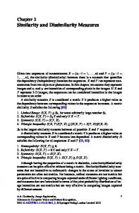
When observing the dendrograms in Fig. 2, one can see they can be divided into two groups from a point of view of their structure. The first group consists of the IOF measure and the Lin measure, the second one of the OF measure and the overlap measure. When looking at the variables in created clusters from a substantive interpretation, the two-cluster solution should be sufficient. There arises a question here, which of groups of measures provides better clusters of variables. Fig. 2: Dendrograms for a set of three-category variables

Source: IBM SPSS, own computations

The clusters provided by the IOF and the Lin measure have a better substantive interpretation than the other ones, i.e. variables in their clusters are ordered more logically. Also, when looking at the dendrograms, the length between first and second level of branching is much bigger by the measures from the first group, which suits for their better distinguishing ability. In the end it was chosen the two-cluster solution provided by the Lin measure, which has the same clusters as the IOF measure. The first cluster deals with 1543


variables concerning the getting a job (A. to get a job, B. to have better salary for the same job, C. to get a leadership, D. to be a director and J. a chance of success). The second cluster consists of variables regarding the getting better position in a job, which you already have: (E. to promote, F. for a salary increase, G. to gain benefits, H. to have authority, I. to keep a job).

Conclusion In this paper, a clustering performance of four similarity measures in categorical variable clustering was examined. There were two main aspects of a comparison. Firstly, the final cluster solutions were evaluated from a point of view of the within-cluster variability; secondly, on a basis of dendrograms and judgments of the researcher. For the analysis, sets of two- and three-categorical variables were chosen. In both datasets, there were not substantial differences among all similarity measures from a point of view of within-cluster variability. When comparing clustering of the overlap measure to the other ones, which are based on frequencies of categories, it had slightly worse results in the dataset with the two-categorical variables and average results in the dataset with the three-categorical variables. However, the crucial difference among the measures is apparent when analyzing their dendrograms. The IOF and the Lin measures provided very good clusters of variables in both datasets from aspects of their substantive interpretation. Therefore, the use of one of these measures is highly recommended for variable clustering. The overlap measure had clusters of unbalanced size and their substantive interpretation is lower than by other measures. The behavior of the OF measure is very difficult to predict, therefore, it cannot be recommended for categorical variable clustering as well.

Acknowledgment This work was supported by the University of Economics, Prague under Grant IGA F4/104/2014.

References Chavent, M., Kuentz, V., Saracco, J. (2010). A Partitioning Method for the Clustering of Categorical Variables. In Locarek-Junge, H., Weihs, C. (Eds.), Classification as a Tool for Research. Studies in Classification, Data Analysis, and Knowledge Organization. Springer, Berlin Heidelberg, 91-99. Greenacre, M. J. (2010). Correspondence analysis. Wiley interdisciplinary reviews: Computational statistics, September/October 2010, 2(5), 613–619. 1544


Frolov, A. A., Húsek, D., Polyakov, P. Y. (2014). Two expectation-maximization algorithms for Boolean factor analysis. Neurocomputing, 130(SI), 83-97. Jolliffe, I. T. (2002). Principal component analysis (2nd ed.). New York: Springer. Sparck-Jones, K. (1972). A statistical interpretation of term specificity and its application in retrieval. Journal of Documentation, 28(1), 11-21. Later: Journal of Documentation, 60(5) (2002), 493-502. Lin, D. (1998). An information-theoretic definition of similarity. In ICML '98: Proceedings of the 15th International Conference on Machine Learning. San Francisco: Morgan Kaufmann Publishers Inc., 296-304. Palla, K., Knowles, D. A., Ghahramani, Z. (2012). A nonparametric variable clustering model. In Advances in Neural Information Processing Systems. Prokop, M., Řezanková, H. (2011). Data dimensionality reduction methods for ordinal data. In Löster T., Pavelka T. (Eds.), International Days of Statistics and Economics. Melandrium, Slaný, 523-533. ISBN 978-80-86175-77-5. Řezanková, H., Löster, T. (2013). Cluster analysis of households characterized by categorical indicators. E+M Ekonomie a Management, 16(3), 139-147. Řezanková, H., Löster, T., & Húsek, D. (2011). Evaluation of categorical data clustering. In Mugellini, E, Szczepaniak, P. S., Pettenati, M. C. et al. (Eds.), Advances in Intelligent Web Mastering 3. Berlin: Springer Verlag, 173-182. ISBN 978-3-642-18028-6. Šulc, Z. (2014). Comparison of new approaches in nominal data clustering. In Sborník prací vědeckého semináře doktorského studia FIS VŠE. Praha: Oeconomica, 214-223. ISBN 97880-245-2010-0.

Contact Zdeněk Šulc University of Economics, Prague, Dept. of Statistics and Probability W. Churchill sq. 4, 130 67 Prague 3, Czech Republic [email protected]

1545