Simple Algorithms for Peak Detection in Time-Series Girish Keshav Palshikar Tata Research Development and Design Centre (TRDDC) 54B Hadapsar Industrial Estate Pune 411013, India. Email:
[email protected]
1
Simple Algorithms for Peak Detection in Time-Series Abstract: Identifying and analyzing peaks (or spikes) in a given time-series is important in many applications. Peaks indicate significant events such as sudden increase in price/volume, sharp rise in demand, bursts in data traffic etc. While it is easy to visually identify peaks in a small univariate time-series, there is a need to formalize the notion of a peak to avoid subjectivity and to devise algorithms to automatically detect peaks in any given time-series. The latter is important in applications such as data center monitoring where thousands of large time-series indicating CPU/memory utilization need to be analyzed in real-time. A data point in a time-series is a local peak if (a) it is a large and locally maximum value within a window, which is not necessarily large nor globally maximum in the entire time-series; and (b) it is isolated i.e., not too many points in the window have similar values. Not all local peaks are true peaks; a local peak is a true peak if it is a reasonably large value even in the global context. We offer different formalizations of the notion of a peak and propose corresponding algorithms to detect peaks in the given time-series. We experimentally compare the effectiveness of these algorithms.
Keywords:
Time-series, Peak detection, Burst detection, Spike detection
1. INTRODUCTION Identifying and analyzing peaks (also called spikes) in a given time-series is an important in many applications, because peaks are useful topological features of a time-series. In power distribution data, peaks indicate sudden high demands. In server CPU utilization data, peaks indicate sharp increase in workload. In network data, peaks correspond to bursts in traffic. In financial data, peaks indicate abrupt rise in price or volume. Troughs can be considered as inverted peaks and are equally important in many applications. Many other application areas – e.g., bioinformatics (Azzini et al (2004)), mass spectrometry (Coombes et al (2005)), signal processing (Jordanov, Hall and Kastner (2002), Harmer et al (2008)), image processing (Ma1, van Genderen1 and Beukelman (2005)), astrophysics (Zhu and Shaha 2003) – require peak detection. We distinguish between peaks (which are high values with sharp rise followed quickly by sharp fall implying a narrow base width) and bursts (which are relatively wide contiguous regions of high values). Thus a burst consists of a wide region of high values with sharp falls on 2
either side, whereas a peak is a very narrow region (only a few points) of high values with sharp falls on either side. We formalize these notions below.
After the peaks are detected, analysis of these peaks consists of many tasks such as identifying periodicity of peaks (Vlachos, Meek, Vagena and Gunopulos (2004)), forecasting the time of occurrence and value of the next peak (Choi, Park, Kim and Kim (1996)) and identifying dependencies among peaks of two or more time-series (e.g., in a multivariate time-series).
While it is easy to visually identify peaks in a small univariate time-series, there is a need to formalize the notion of a peak to avoid subjectivity and to devise algorithms to automatically detect peaks in any given time-series. The latter is important in applications such as data center monitoring where thousands of large time-series indicating CPU/memory utilization of thousands of servers need to be analyzed in real-time.
In this paper, we propose several different ways of formalizing the notion of a peak. We present several different algorithms, each based on a specific formalization of the notion of a peak, to detect all peaks in the given time-series. We discuss experimental evaluation of these algorithms. We also provide a comparison of the proposed algorithms among each other and with those in the related literature.
2. RELATED WORK Peak detection is a common task in time-series analysis and signal processing. Standard approaches to peak detection include (i) using smoothing and then fitting a known function (e.g., a polynomial) to the time-series; and (ii) matching a known peak shape to the time-series. Another common approach to peak-trough detection is to detect zero-crossings (i.e., local maxima) in the differences (slope sign change) between a point and its neighbours. However, this detects all peaks-troughs, whether strong or not. To reduce the effects of noise, it is required that the local signal-to-noise ratio (SNR) should be over a certain threshold; see Nijm et al (2007) and Jordanov, Hall and Kastner (2002). The key question now is how to set the correct threshold so as to minimize false positives. Ma, van Genderen and Beukelman (2005) compute 3
the threshold automatically by adapting it to the noise levels in the time-series as h = (max + abs_avg)/2 + K * abs_dev, where max is the maximum value in the time-series, abs_avg is the average of the absolute values in the time-series, abs_dev is the mean absolute deviation and K is a user-specified constant.
Azzini et al (2004) analyze peaks in gene expression microarray time-series data (for malaria parasite Plasmodium falciparum) using multiple methods; each method assigns a score to every point in the time-series. In one method, the score is the rate of change (i.e., the derivative) computed at each point. In another method, the score is computed as the fraction of the area under the candidate peak. Top 10 candidate peaks are selected for each method; peaks detected by multiple methods are chosen as true peaks. The detected peaks are used to identify genes; SVM are then used to assign a functional group to each identified gene.
Key problems in peak detection are noise in the data and the fact that peaks occur with different amplitudes (strong and weak peaks) and at different scales, which result in a large number of false positives among detected peaks. Based on the observation that peaks in mass spectroscopy data have characteristic shapes, Du, Kibbe and Lin (2006) propose a continuous wavelet transform (CWT) based pattern-matching algorithm for peak detection. 2D array of CWT coefficients is computed (using a Mexican Hat mother wavelet which has the basic shape like a peak) for the time-series at multiple scales and “ridges” in this wavelet space representation are systematically examined to identify peaks. Coombes et al (2005) and Lange et al (2006) present other approaches for peak detection using wavelets and their applications to analyze spectroscopy data.
Zhu and Shasha (2003) propose a wavelet-based burst (not peak) detection algorithm. The wavelet coefficients (as well as window statistics such as averages) for Haar wavelets are organized in a special data structure called the shifted wavelet tree (SWT). Each level in the tree corresponds to a resolution or time scale and each node corresponds to a window. By automatically scanning windows of different sizes and different time resolutions, the bursts can be elastically detected (appropriate window size is automatically decided). Zhu and Shasha 4
(2003) apply their technique to detecting Gamma Ray bursts in real-time in the Milagro astronomical telescope, which vary widely in their strength and duration (from minutes to days).
Harmer et al (2008) propose a momentum-based algorithm to detect peaks. The idea is compute velocity (i.e., rate of change) and momentum (i.e., product of value and velocity) at various points. A “ball” dropped from a previously detected peak will gain momentum as it climbs down and lose momentum as it climbs the next peak; the point where it comes to rest (loses all its momentum) is the next peak. Simple analogs of the laws in Newtonian mechanics are proposed (e.g., friction) to compute changes in momentum as the ball traverses the time-series.
Vlachos et al (2004) describe a moving average based algorithm for burst (not peak) detection; our peak function S2 is closely related to this algorithm. The time-series is smoothed using a moving average filter and values which are larger than x times the standard deviation of the entire (smoothed) time-series are considered as peaks; x is typically between 1.5 to 2.0. The extent of smoothing is decided using domain knowledge (e.g., 30 points for daily data). See also Vlachos et al (2008) for closely related work, application to burst detection in real-time streaming data and analysis of correlations between bursts.
3. PROBLEM FORMALIZATION Let T = x1, x2, …, xN be a given univariate uniformly sampled time-series containing N values. Without loss of generality, the time instants are assumed to be 1, 2, …, N (i.e., the time-series T is uniformly sampled). Let xi be a given ith point in T. Let S be a given peak function, which associates a score (which is a non-negative real number) S(i, xi, T) with ith element xi of the given time-series T. A given point xi in T is a peak if S(i, xi, T) , where is a user-specified (or suitably calculated) threshold value. The important question is: how to compute the function S? We provide different characterizations of the peak function S.
We begin with the observation that a peak is clearly a local phenomenon, although a local peak may not be accepted as a true peak in the light of other peaks in the time-series. A data point in a time-series is a local peak if (a) it is a large and locally maximum value within a window; the 5
value need not necessarily be large nor globally maximum in the entire time-series; and (b) it is isolated i.e., not too many points in the window have similar values. Not all local peaks are true peaks; a local peak is a true peak if it is a reasonably large value even in the global context. We offer different formalizations of the notion of a peak and propose corresponding algorithms to detect peaks in the given time-series.
We first propose several different ways to compute the function S, which captures the “spikiness” of the point xi in the local context. We then discuss how locally detected peaks (using the function S) can be validated in the time-series as a whole. In the following, we assume that k > 0 is a given integer. Let N+(k,i,T) = the sequence of k right temporal neighbours of xi i.e., k points immediately following the ith point xi in T. N(k,i,T) is defined similarly as the set of k left (previous) temporal neighbours of xi. Let N(k,i,T) = N+(k,i,T) N(k,i,T) denote the sequence of 2k points around the ith point (without the ith point itself) in T ( denotes concatenation). Let N(k,i,T) = N+(k,i,T) {xi} N(k,i,T). For clarity, the definitions below generally assume that k < i < N – k; each definition can be easily modified to cover other values of i towards the beginning and end of the time-series.
1. For a given point xi in T, the following function S1 computes the average of (i) the maximum among the signed distances of xi from its k left neighbours and (ii) the maximum among the signed distances of xi from its k right neighbours. Low values of k (e.g., 3 to 5) are usually suitable, if most peaks are “thin”. Values of S1(k,i,xi,T) indicate the “significance” of the height of the peak at the ith time instant. S1 ( k , i , x i , T )
max{xi xi 1 , xi xi 2 ,, xi xi k } max{xi xi 1 , xi xi 2 ,, xi xi k } 2
2. Function S2 computes the average of (i) the average of the signed distances of xi from its k left neighbours and (ii) the average of the signed distances of xi from its k right neighbours.
( xi xi 1 xi xi 2 xi xi k ) ( xi xi 1 xi xi 2 xi xi k ) k k S 2 ( k , i , xi , T ) 2 3. Function S3 computes the average signed distance of the ith value xi in T from the average value of its k temporal neighbours. 6
x xi 2 ... xi k x xi 2 ... xi k xi i 1 xi i 1 k k S 3 ( k , i, xi , T ) 2
4. Entropy of any sequence of M values A = is defined as follows: M
H w ( A) p w (ai ) log( p w (ai ))
i 1
where pw(ai) is an estimate of the probability density at ai. The kernel density technique (also called Parzen window) can be used (Wand and Jones (1995)) to estimate the probability density p(ai) at ith value ai in the given sequence A: p w (ai )
1 M ai ai w
M
ai a j a i i w
K a j 1
where K is a suitable kernel function and w > 0 is a given integer. Subscript w in H and p indicates the width parameter used in kernel density estimation. Epanechnikov and Gaussian are two well-known kernel functions (defined below):
3 1 x2 4 0
K ( x)
K ( x)
1 2
e
if | x | 1 otherwise
1 2 x 2
Function S4 computes the difference in the entropy of the two sequences N(k,i,T) and N(k,i,T), which gives an idea of how “influential” or significant xi is in this window. Gaussian kernel is used to compute the density estimate. S 4 (k , w, i, xi , T ) H w ( N (k , i, T )) H w ( N (k , i, T ))
5. Another idea is that a peak would be an “outlier” when considered in the local context of a window of 2k points around it. While there are a large number of sophisticated approaches for outlier detection (Barnett and Lewis (1994)), considering the need for efficiency and ability to work with small data (2k points), we use either one of the following well-known techniques. Let m, s denote the mean and standard deviation of the 2k data points in N(k,i,T) around xi.
7
(a) The ith point xi is a peak if (i) xi m and (ii) |xi – m| 3s. Assuming that the 2k values in N(k,i,T) are normally distributed with mean m and standard deviation s, by the wellknown normal probability rule, P[ –3s < xi – m < –3s] = 0.997. Hence, if |xi – m| 3s then the value xi is clearly rare. Since the data in N(k,i,T) may not always be normally distributed, we propose the following non-parametric technique. (b) Chebyshev Inequality states that for a random variable X with mean and standard deviation , and for any positive number h, P[|X - | < h] 1 – 1/h2 i.e., P[|X - | h] < 1/h2. Applying this to our case (and using m and s as estimators of and ), P[|xi - m| hs] < 1/h2; e.g., h = 3 gives P[|xi - m| 3s] < 0.111. Chebyshev Inequality is nonparametric i.e., it does not assume any particular distribution for the values of the random variable X. Another decision rule for whether xi is a peak or not is as follows: the ith point xi is a peak if (i) xi m and (ii) |xi – m| hs, for some suitably chosen h > 0. Using each of the above peak functions, we could easily write an algorithm to detect all peaks in the given time-series T. We show below the algorithm that uses the peak function S1 (other peak detection algorithms are very similar, except that each uses a different peak function). The peak function S1 computes its value at each point using the local window (context) of size 2k around that point. All points where the peak function has a positive value are candidate peaks. We rule out some of these locally detected peaks using the global context (time-series as a whole) as follows. We compute the mean m and standard deviation s of all positive values of the peak function and then retain only those points xi in the time-series which satisfy the condition S1(k,i,xi,T) – m > h * s, where h is a user-specified constant. A simple post-processing (used in all algorithms) involves removing peaks if they are “too near” to each other (e.g., within the same window of size k).
8
algorithm peak1 // one peak detection algorithms that uses peak function S1 input T = x1, x2, …, xN, N
// input time-series of N points
input k
// window size around the peak
input h
// typically 1 h 3
output O
// set of peaks detected in T
begin O=
// initially empty
for (i = 1; i < n; i++) do a[i] = S1(k,i,xi,T); // compute peak function value for each of the N points in T end for Compute the mean m and standard deviation s of all positive values in array a; for (i = 1; i < n; i++) do // remove local peaks which are “small” in global context if (a[i] > 0 && (a[i] – m) >( h * s)) then O = O {xi}; end if end for Order peaks in O in terms of increasing index in T // retain only one peak out of any set of peaks within distance k of each other for every adjacent pair of peaks xi and xj in O do if |j – i| k then remove the smaller value of {xi, xj} from O end if end for end 4. EXPERIMENTAL EVALUATION In this section, we present a quick comparison of the proposed algorithms on a sample timeseries. The time-series consists of annual sunspot data for years 1700 to 2008 and is obtained from the following web-site: ftp://ftp.ngdc.noaa.gov/STP/SOLAR_DATA/SUNSPOT_NUMBERS/YEARLY.PLT As seen, entropy-based peak function S4 has detected all peaks; S5 has also done quite well but the other peak functions have missed some peaks. Note that there are no false positives. Fig. 2 shows a much noisier time-series, where we have got similar results (S4, S5 worked well).
9
(a) S1: k=5 h=1.5
(b) S2: k=5 h=1.5
(c) S3: k=5 h=1.5
(d) S4: k=5 w=5 h=1.5
(e) S5: k=5 h=1.5
Fig.1. Peaks detected in the annual sunspot number time-series using proposed algorithms (first k and last k points are not analyzed for peaks).
10
(b) S2: k=5 h=1.5
(a) S1: k=5 h=1.5
(d) S4: k=15 w=3
(c) S3: k=5 h=1.5
(e) S5: k=10 h=1.5
Fig.2. Peaks detected in a time-series of 480 points using proposed algorithms (first k and last k points are not analyzed for peaks).
11
5. CONCLUSIONS AND FURTHER WORK In this paper, we have proposed a formal characterization of the notion of a peak in a time-series and have presented several algorithms for peak detection. We also presented a quick experimental evaluation of the proposed algorithms. The algorithms work on the raw time-series data and do not need any pre-processing such as smoothing, thereby eliminating some subjective aspects. We are working on a more in-depth evaluation as well on deploying the peak detection techniques in different applications. Often an element of experimentation is involved in choosing the right values of the parameters (e.g., k) of the proposed peak detection algorithms. We have identified some useful heuristics to automatically select the right parameter values. We are working on peak detection in an online setting, which is important in some applications.
Acknowledgements. I thank Prof. Harrick Vin for his guidance and encouragement throughout this work. Thanks to Manoj Jain, Navneet Rao, Shivam Sahai and other colleagues in TRDDC for their help and useful discussions. Sincere thanks to Dr. Manasee Palshikar for her support.
References Azzini I., Dell’Anna R., Ciocchetta F., Demichelis F., Sboner A., Blanzieri E., Malossini A. (2004), “Simple Methods for Peak Detection in Time Series Microarray Data”, Proc. CAMDA’04 (Critical Assessment of Microarray Data). Barnett V., Lewis T. (1994), Outliers in Statistical Data, 3/e, Wiley Publishers. Choi J.-G., Park J-K., Kim K.-H., Kim J.-C. (1996), “A Daily Peak Load Forecasting System using a Chaotic Time Series”, Proc. Int. Conf. on Intelligent Systems Applications to Power Systems, pp. 283 – 287. K.R. Coombes et al. (2005), “Improved Peak Detection and Quantification of Mass Spectrometry Data Acquired from Surface-enhanced Laser Desorption and Ionization by Denoising Spectra with the Undecimated Discrete Wavelet Transform, Proteomics, 5, 4107–4117. Du P., Kibbe W.A., Lin S.M. (2006), “Improved Peak Detection in Mass Spectrum by Incorporating Continuous Wavelet Transform-based Pattern Matching”, Bioinformatics, vol. 22, no. 17, pp. 2059 – 2065. Jordanov V.T., Hall D.L., Kastner M. (2002), “Digital Peak Detector with Noise Threshold”, Proc. IEEE Nuclear Science Symposium Conference, vol. 1, pp. 140 – 142. 12
Harmer K., Howells G., Sheng W., Fairhurst M., Deravi F. (2008), “A Peak-Trough Detection Algorithm Based on Momentum”, Proc. IEEE Congress on Image and Signal Processing (CISP), pp. 454 – 458. Kleinberg J. (2002), “Bursty and Hierarchical Structure in Streams”, Proc. 8th ACM SIGKDD Conf., ACM Press, pp. 91–101. Lange E., Gropl C., Reinert K., Kohlbacher O., Hildebrandt A., (2006), “High Accuracy Peak Picking of Proteomics Data using Wavelet Techniques”, in Proceedings of Pacific Symposium on Biocomputing 2006, Maui, Hawaii, USA, pp. 243–254. Ma1 M., van Genderen1 A., Beukelman P. (2005), “Developing and Implementing Peak Detection for Real-Time Image Registration”, Proc. 16th Annual Workshop on Circuits, Systems and Signal Processing (proRISC2005), pp. 641 – 652. Nijm G. M., Sahakian A. V., Swiryn S., Larson A. C. (2007), “Comparison of Signal Peak Detection Algorithms for Self-Gated Cardiac Cine MRI”, Computers in Cardiology 2007. Vlachos M., Meek C., Vagena Z., Gunopulos D. (2004), “Identification of Similarities, Periodicities and Bursts for Online Search Queries”, Proc. SIGMOD 2004 Conf., ACM Press, pp. 131–142. Vlachos M., Wu K.-L., Chen S.-K., Yu P.S. (2008), “Correlating Burst Events on Streaming Stock market Data”, Data Mining and Knowledge Discovery, vol. 16, pp. 109 – 133. Wand M.P., Jones M.C. (1995), Kernel Smoothing, Chapman and Hall. Zhu Y., Shasha D. (2003), “Efficient Elastic Burst Detection in Data Streams”, Proc. SIGKDD 2003 Conf., ACM Press, pp 336–345.
13