When analyzing handwritten signatures using a computer, a certain amount of variation within any par- ticular class is to be expected. Successful recognition.
Simple Distances Between Handwritten Signatures J.R. Parker Laboratory for Computer Vision Department of Computer Science University of Calgary
Abstract When analyzing handwritten signatures using a computer, a certain amount of variation within any particular class is to be expected. Successful recognition demands that this variation be less than that between two different signatures. This paper describes three simple ways to compare signatures that do not use any complicated or derivative feature measurements, each of which defines a distance between signatures that allows individual variation.
50 signatures overlaid. The variation in position of related pixels is over 10%.
FIGURE 1.
1. Introduction The use of handwritten signatures to verify and individual’s identity is older than photography. Common wisdom and practice has it that signatures are unique, and that human experts can match two signatures well enough for most practical purposes. A difficulty with automatic signature verification, the comparison of an input signature with a known file sample signature using computer algorithms, is that two signatures are never exactly the same, not even for the same person under identical circumstances. Thus, the signatures are never compared directly. Signature verification is frequently performed by making various measurements on a digitized image[4,5,10] and subjecting these to a classifier, like a neural net or support vector machine[1,2,3]; the measurements are called features, and often a great many are used, creating a feature vector. The features are numerical values, and will vary somewhat between instances created by the same writer. The hope is that the features will vary more for two different writers (between-class variance) than for the same writer (in-class variance). It has been claimed that signatures are written with a great deal of consistency, especially with respect to orientation and scale (for example [11]). This may be true if the writer is constrained to use a particular form, but is not sufficiently true in unconstrained cases to yield consistent sets of features for recognition. Figure 1 shows a set of 50 signatures drawn freehand on a Wacom data tablet. The variation can be seen clearly, but is difficult
to measure in any really meaningful way. For example, the maximum distance between temporally related points (points the same time from the time of the first pen down) is 76 pixels, or 19% of the signature width. The maximum distance between any two closest points is 22 pixels (5.5% of width). Its not clear what any of this really means. or how it could be used to verify the identity of the writer. What is clear is that if, as is claimed, in-class signatures are in some sense more similar to each other than they are to out-class signatures, then there is some obvious (at least to the human visual system) measure that minimizes the small variations normal to signatures and uses larger ones to make distinctions.
2. Measuring Distance How can it be decided automatically that some variation from a template signature is natural, while another variation indicates that two distinct signatures are involved? Usually by looking at what ‘distances’ between signatures written by the same writer are typical, and comparing to the distances obtained between classes. By ‘distance’, we could mean any number of things, usually involving feature vectors and somewhat complicated measurements. The work described here is an effort to determine whether simple, relatively obvious distances can yield good results. Again, many different things may be meant by ‘relatively obvious’. What is meant here is distance will be
computed in a Euclidean fashion, from points in two dimensional geometric space. 2. 1 Temporal Distance If two signatures are instances of the same class, it should be true that points on each that were sampled at the same time relative to the initial pen down time should be near to each other spatially [7]. To measure this, a standard coordinate system is needed; the centroid of the signature should serve very well as the origin. It is also necessary to know at what relative time each pixel was drawn, and for this the signature must have been captured using a Wacom data tablet or similar device. These return pen coordinates at regular sampling intervals. Times associated with points between two sampled coordinates can be interpolated. There are issues around scale to be addressed as well. The basic process involved in computing temporal distance is as follows: The signature being validated is S; the exemplar being compared against currently is Ei. 1. Rescale Ei to the same size as S, but do not alter the aspect ratio of Ei. Some size variation will therefore remain. 2. Because Ei has changed size, the time needed to draw it should change also. Based on the ratio of old arc length to new, compute the new value for the time needed to draw Ei, Te [6]. 3. Convert the coordinates for both S and Ei from those relative to the capture tablet to those relative to the centroid of each signature. 4. Now divide the time interval needed to draw S into a fixed number of smaller intervals- we use 250 such subintervals. For each subinterval, calculate the (x,y) position of the pen for both S and Ei. Determine the distance between these two points, and accumulate the sum of these distances in d.
The distance between S and Ei is d/250, or the average position error per subinterval.
d0
2. 2 Global Relative Distance While any two instances of a signature will differ from each other, they should be nearer to each other in some sense than to instances of different signatures. A measurement based on this idea would involve finding the distance from a black pixel in one signature to the nearest black pixel in the other. Of course, it would probably be best to find the difference between corresponding pixels in the two images, but the cost of doing this would be prohibitive, and the improvement may not be significant. Again, as in temporal distance, a common coordinate system must be used, and a common scale must be agreed on. The same method as described in section 2.1 is used here, in which a common scale is agreed on and the coordinate system is centroid based. Next the distance is calculated using a distance transform. Consider the signature image S. The distance transform is an image D the same size as S in which the value of each pixel Dij is the distance from the pixel Sij to the nearest object pixel. We used the 8-distance, because it is a simple matter to compute the entire transform in two passes through the image[8,9]. The distance Ei-S for an exemplar image Ei is found by computing D as described and accumulating the sum of all Dij where Eij is an object pixel. This is essentially the distance from each object pixel in Ei to the nearest object pixel in S. We need to compute also the distance S-Ei, which uses the distance transform of Ei in a symmetrical manner to the above. The distance between Ei and S is the product of these two distances. The distance images can be computed in advance and stored instead using the raw images and recomputing the distances each time. 2. 3 Multiple Signature Masks Slight variations in signatures can be thought of as noise, and a standard method for dealing with noisy data is to average multiple samples. Combine this idea with
d0
d1
d0, the distance between the initial points on the two signatures. FIGURE 2.
After a small time increment, both pens move. d1 is the distance between the new points.
How temporal distance is calculated. After the signatures are scaled, each is broken into 250 pieces by time taken to draw. The distance between the two signatures after each interval is summed.
Similar signatures should be nearer to each other after each interval.
that of global relative distance (Section 2.2 above) and we get the multiple signature mask algorithm. Imagine that for writer A we have 50 signature samples. A signature mask is produced by scaling all images to a standard size, and then creating a new image (the mask image) in which a pixel is set to object level if that pixel is an object pixel in any of the samples. The pixel is set to background level otherwise. In a multiple signature mask each mask pixel is incremented for each corresponding object pixel in any sample image. There are no longer individual exemplar images, only one mask image for each class. To compute the distance between a sample S and a class represented by mask image M, simply sum into D the mask pixel values Mij that correspond to object pixels in the image S. Pixels Mij that correspond to background (I.E. were never set in any example image for that class) result in a decrease of the sum D - we use a value of -5, but this is an arbitrary penalty and the optimal value is not known. The final value of D is a similarity value rather than a distance, since larger values correspond to more similar object.
3. Experimental Protocol The data used for testing the verification methods consists of a total of 690 signatures, which consists of 50 samples (actually between 46-50 samples) of 14 individuals. These signatures were captured using the Wacom data tablet and image data was generated from the data points for the image based methods. Because of the relatively small amount of data available, a ‘leave-one-out’ protocol was used. A database of signatures was constructed for each trial, omitting the target in each case. In other words, the set of exemplars never includes the signature being evaluated. However, every signature is compared against all others, both in class and out-class, and the smallest single distance (or largest similarity value) represents the correct classification. A confusion matrix is created in each case, showing all of the information available for the trials. Correct classifications, false positives, and false negatives are all present. 3. 1 Results and Conclusions To this point three different methods for comparing signatures have been discussed. Using the protocol
(a)
2
2
1
2
1
4
5
4
4
3
1
2
4
2
3
2
2
1
3
3
1
1
1
2
5
3
1
4
2
1
(b)
(a) Calculation of the distance from a simple distance map (Darker pixels are more distant from an object pixel). The map of the exemplar is overlaid with the signature, and a score is found by incrementing a counter by the distance found whenever the line passes over a pixel in the mask. (b) A mask image consists of a count of the number of times that each pixel is object level in all exemplars. Similarity is the sum of all pixels touched by a given signature; empty pixels count against, reducing the similarity value.
FIGURE 3.
Confusion Matrix for Temporal Distance Overall: 92.7% 0 1 2 3 4 5 6 7 8 9 10 11 12 13 0 50 0 0 0 0 0 0 0 0 0 0 0 0 0 1 0 49 0 0 0 1 0 0 0 0 0 0 0 0 2 0 0 45 0 0 0 0 4 0 0 0 0 0 0 3 1 0 0 46 0 0 0 0 0 0 0 0 2 0 4 0 0 1 0 49 0 0 0 0 0 0 0 0 0 5 1 1 0 0 0 48 0 0 0 0 0 0 0 0 6 0 0 0 0 0 0 49 1 0 0 0 0 0 0 7 0 0 0 0 0 0 1 47 0 0 0 0 0 0 8 1 0 0 0 0 0 1 3 42 0 0 2 0 1 9 0 0 0 0 0 0 1 1 0 44 1 0 0 0 10 0 0 0 0 0 0 0 2 0 0 45 2 0 0 11 2 1 0 0 0 0 1 3 3 0 0 38 1 0 12 1 1 0 2 0 0 0 2 2 0 0 1 40 0 13 0 0 0 0 0 0 1 1 0 0 0 0 0 48 Confusion Matrix for Global Relative Distance Overall: 97.1% 0 1 2 3 4 5 6 7 8 9 10 11 12 13 0 50 0 0 0 0 0 0 0 0 0 0 0 0 0 1 0 50 0 0 0 0 0 0 0 0 0 0 0 0 2 1 0 49 0 0 0 0 0 0 0 0 0 0 0 3 1 0 1 45 1 0 0 0 0 0 2 0 0 0 4 0 0 0 0 50 0 0 0 0 0 0 0 0 0 5 0 0 0 0 0 50 0 0 0 0 0 0 0 0 6 1 0 0 0 0 0 49 0 0 0 0 0 0 0 7 3 0 0 0 0 0 0 47 0 0 0 0 0 0 8 0 0 0 0 0 0 0 0 50 0 0 0 0 0 9 3 0 0 0 0 0 0 0 0 47 0 0 0 0 10 1 0 0 0 0 0 0 0 0 0 49 0 0 0 11 1 0 0 0 0 0 0 0 0 0 0 49 0 0 12 1 2 0 0 0 1 0 0 0 0 0 1 45 0 13 0 0 0 0 0 0 0 0 0 0 0 0 0 50 described in this section, the results for all methods are as shown in Figure 4 as confusion matrices. Every row and column represents a signature class. Each row in the matrix sums to the total number of elements in the class, and off-diagonal elements in a row represent false rejections. Off-diagonal elements in a column represent false acceptances. Foe example, consider class 5 in the temporal distance matrix; 48/50 were correctly classified, one was classed as class 0 and one as class 1 for a total of 2 false rejections. A false acceptance of a class 1 signature occurred. It is obvious that, with a method that works correctly on all available data, it is difficult to suggest an improvement. As a student in the lab pointed out when confronted with a diagonal confusion matrix, ‘I guess we need more data.’ He is exactly correct. And yet the goal was not to produce an ‘ideal’ signature recognizer or verification system. It was simply to demonstrate that signatures can be distinguished using simple means, direct comparisons and straightforward distance computations.
Figure 4 - Results for the three signature recognition techniques discussed. Left - temporal distance. Left and below - Global relative distance. Below - Multiple signature masks, which correctly recognizes all signatures in our data set.
Confusion Matrix for Multiple Signature Masks Overall: 100% 0 1 2 3 4 5 6 7 8 9 10 11 12 13 0 50 0 0 0 0 0 0 0 0 0 0 0 0 0 1 0 50 0 0 0 0 0 0 0 0 0 0 0 0 2 0 0 50 0 0 0 0 0 0 0 0 0 0 0 3 0 0 0 50 0 0 0 0 0 0 0 0 0 0 4 0 0 0 0 50 0 0 0 0 0 0 0 0 0 5 0 0 0 0 0 50 0 0 0 0 0 0 0 0 6 0 0 0 0 0 0 50 0 0 0 0 0 0 0 7 0 0 0 0 0 0 0 50 0 0 0 0 0 0 8 0 0 0 0 0 0 0 0 50 0 0 0 0 0 9 0 0 0 0 0 0 0 0 0 50 0 0 0 0 10 0 0 0 0 0 0 0 0 0 0 50 0 0 0 11 0 0 0 0 0 0 0 0 0 0 0 50 0 0 12 0 0 0 0 0 0 0 0 0 0 0 0 50 0 13 0 0 0 0 0 0 0 0 0 0 0 0 0 50 It is not at all clear that the multiple signature mask technique can be used in practical situations. This needs to be explored further, but at the present time the computation is slow, and there may be a practical limit to how many signatures can be distinguished. The global relative distance method works as well as most published algorithms, and has the advantage of being quite simple and obvious. It, too, may be too slow for most real applications. The point, however, has been made. A simple direct comparison is possible, and has a high success rate.
4. References [1] M. Ammar, Y. Yoshida, and T. Fukumura, Off-line Preprocessing and Verification of Signatures, International Journal of Pattern Recognition and Artificial Intelligence, Vol. 2, No. 4, 1988. Pp. 589-602. [2] V. Anastassopoulos and A. Venetsanopoulos, The Classification Properties of the Pecstrum and Its Use for Pattern Identification, Circuits Systems Signal Processing Vol. 10 No. 3, 1991. Pp. 293-326
[3] R. Bajaj and S. Chaudhury, Signature Verification Using Multiple Neural Classifiers, Pattern Recognition, Vol 30, No 1, 1997. pp. 1-7. [4] K. Huang and H. Yan, On-line signature Verification Based on Dynamic Segmentation and Global and Local Matching, Optical Engineering, Vol. 34 No. 12, 1995. Pp. 3480-3487. [5] F. LeClerc and R. Plamondon, Automatic Signature Verification: The State Of The Art, International Journal of Pattern Recognition, Vol 8, No 3, 1994. pp. 643-660. [6] R. Martens and L. Claesen, On-Line Signature Verification by Dynamic Time Warping, Proc. 13th ICPR, 1996. Pp. 38-42. [7] M. Munich and P. Perona, Visual Signature Verification Using Affine Arc Length, [8] J.R. Parker, Practical Computer Vision Using C, John Wiley and Sons, New York, N.Y., 1993. [9] J. R. Parker, A Faster Method for Erosion and Dilation of Reservoir Pore Complex Images, Canadian Journal of Earth Sciences, July 1988. [10] J. Riba, A. Carnicer, S. Vallmitjana, and I. Juvells, Methods for Invariant Signature Classification, Proceedings of ICPR 2000, Barcelona, Spain. pp. 957-960. [11] R. Sabourin and G. Genest, An Extended Shadow Code Based Approach for Off-Line Signature Verification: Part I - Evaluation of the Bar Mask Definition, 12th ICPR, Jerusalem, Israel, Oct 9-13, 1994. Pp. 450-453.