Jan 25, 2014 - OC] 25 Jan 2014. Simple Error Bounds for Regularized Noisy Linear Inverse Problems. Christos Thrampoulidis, Samet Oymak and Babak ...
Simple Error Bounds for Regularized Noisy Linear Inverse Problems
arXiv:1401.6578v1 [math.OC] 25 Jan 2014
Christos Thrampoulidis, Samet Oymak and Babak Hassibi Department of Electrical Engineering, Caltech, Pasadena – 91125
Abstract— Consider estimating a structured signal x0 from linear, underdetermined and noisy measurements y = Ax0 +z, ˆ = arg minx {ky− via solving a variant of the lasso algorithm: x Axk2 +λf (x)}. Here, f is a convex function aiming to promote the structure of x0 , say ℓ1 -norm to promote sparsity or nuclear norm to promote low-rankness. We assume that the entries of A are independent and normally distributed and make no assumptions on the noise vector z, other than it being independent of A. Under this generic setup, we derive a general, non-asymptotic and rather tight upper bound on the ℓ2 -norm of the estimation error kˆ x − x0 k2 . Our bound is geometric in nature and obeys a simple formula; the roles of λ, f and x0 are all captured by a single summary parameter δ(λ∂f (x0 )), termed the Gaussian squared distance to the scaled subdifferential. We connect our result to the literature and verify its validity through simulations.
I. I NTRODUCTION A. Motivation We wish to estimate a structured signal x0 ∈ Rn from a vector of compressed noisy linear observations y = Ax0 + z ∈ Rm , where m < n. What makes the estimation possible in the underdetermined regime, is the assumption that x0 retains a particular structure. To promote this structure, we associate with it a properly chosen convex function1 f : Rn → R. As a motivating example, when x0 is a sparse vector, we can choose f (x) = kxk1 . A typical approach for estimating x0 is via convex programming. If f (x0 ) is known a-priori, then the following convex program yields a reasonable estimate: min ky − Axk2 x
s.t. f (x) ≤ f (x0 ).
(1)
ˆ that best fits the vector of It solves for an estimate x observations y while at the same time retains structure similar to that of x0 . Program (1), with f (x) = kxk1 , was introduced in [2] by Tibshirani for estimating sparse signals and is known as the “lasso” in the statistics literature. In practical situations, prior knowledge of f (x0 ) is typically not available, which makes (1) impossible to solve. Instead, one can solve regularized versions of it, like, λ min ky − Axk2 + √ f (x), x m
(2)
Emails: (cthrampo, soymak, hassibi)@caltech.edu. This work was supported in part by the National Science Foundation under grants CCF-0729203, CNS-0932428 and CIF-1018927, by the Office of Naval Research under the MURI grant N00014-08-1-0747, and by a grant from Qualcomm Inc. 1 See [1] for examples and a principled approach to constructing such structure inducing functions.
or min x
τ 1 ky − Axk22 + √ f (x), 2 m
(3)
for nonnegative regularizer parameters λ and τ . Although very similar in nature, (2) and (3) show in general different statistical behaviors [3], [4]. Lagrange duality ensures that there exist λ and τ such that they both become equivalent to the constrained optimization (1). However, in practice, the challenge lies in tuning the regularizer parameters to achieve good estimation, with as low as possible prior knowledge. Assuming that the entries of the noise vector z are i.i.d, it is well-known that a sensible choice of τ in (3) must scale with the standard deviation σ of the noise components [5]– [7]. On the other hand, (2) eliminates the need to know or to pre-estimate σ [3]. This fact was first proven by Belloni et. al. in [3] 2 for the ℓ1 -case f (·) = k · k1 , and has, since then, spurred significant research interest on the analysis of (2). B. Contribution In this work, we derive a simple non-asymptotic upper −x0 k2 bound on the normalized estimation error kˆxkzk of the 2 regularized estimator (2), which holds for arbitrary convex regularizers f (·). We assume that the measurement matrix A has independent zero-mean normal entries of variance 1 m . For the noise vector z, we only require it being chosen independently of A. Our upper bound is a simple function of the number of measurements m and, of a summary parameter δ(λ∂f (x0 )), termed the Gaussian squared distance; δ(λ∂f (x0 )) captures the structure induced by f (·), the particular x0 we are trying to recover and the value of the regularizer parameter λ. For example, when we are interested in a sparse signal, the structure is captured by f (·), whereas the actual sparsity level (i.e. how many entries are zero) is captured by x0 . (Thus δ(λ∂f (x0 )) is the same for all k-sparse x0 ). In recent works [1], [4], [8], [9], δ(λ∂f (x0 )) has been calculated for a number of practical regularizers f (·); making use of these results, translates our bound to explicit formulae. Finally, the constants involved in our result are small and nearly accurate. As a byproduct, our bound provides a guideline on the important practical problem of optimally tuning the regularizer parameter λ. 2 Belloni et. al [3] refer to (2) as the “square-root lasso” to distinguish from the “standard lasso” estimator (3). The authors in [4] refer to the two estimators in (2) and (3) as the ℓ2 -lasso and ℓ22 -lasso, respectively.
C. Related work There is a significant body of research devoted to the performance analysis of lasso-type estimators, especially in the context of sparse recovery. A complete review of this literature is beyond the scope and the space of the current paper. Our result complements and extends recent work in [4], [10]–[12]. The authors in [10] obtain an explicit expression for the normalized error of (3), in an asymptotic setting. [11] proposes a framework for the analysis of lassotype algorithms and relies on it to perform a precise analysis of the (worst-case) estimation error of (1) for f (·) = k·k1 . A generalization of this analysis to arbitrary convex regularizers and an extension to the regularized problem (2) was provided in our work [4]. In contrast to the present paper, the bounds in [4], [11] require stronger assumptions, namely, an i.i.d. Gaussian noise vector z and an asymptotic setting where m is large enough. Our latest work [12] successfully relaxes both those assumptions and derives sharp bounds on the estimation error of the constrained lasso (1). The result presented in the current paper is a natural extension of that, to the more challenging, and practically important, ℓ2 -regularized lasso problem (2). In the context of sparse estimation, our bound recovers the order of best known result in the literature [3], and improves on the constants that appear in it. See Section III-C for a more elaborate discussion on the relation to these works. II.
PRELIMINARIES
For the rest of the paper, let N (µ, σ 2 ) denote the normal distribution of mean µ and variance σ 2 . Also, to simplify notation, let us write k · k instead of k · k2 . A. Convex geometry 1) Subdifferential: Let f : Rn → R be a convex function and x0 ∈ Rn be an arbitrary point that is not a minimizer of f (·). The subdifferential of f (·) at x0 is the set of vectors, � ∂f (x0 ) = s ∈ Rn |f (x0 + w) ≥ f (x0 ) + sT w, ∀w ∈ Rn .
∂f (x0 ) is a nonempty, convex and compact set [13]. It, also, does not contain the origin since we assumed that x0 is not a minimizer. For any nonnegative number λ ≥ 0, we denote the scaled (by λ) subdifferential set as λ∂f (x0 ) = {λs|s ∈ ∂f (x0 )}. Also, for the conic hull of the subdifferential ∂f (x0 ), we write cone(∂f (x0 )) = {s|s ∈ λ∂f (x0 ), for some λ ≥ 0}. 2) Gaussian squared distance: Let C ⊂ Rn be an arbitrary nonempty, convex and closed set. Denote the distance of a vector v ∈ Rn to C, as dist(v, C) = mins∈C kv − sk. Definition 2.1 (Gaussian distance): Let h ∈ Rn have i.i.d N (0, 1) entries. The Gaussian� squared distance of a set C ⊂ � Rn is defined as δ(C) := Eh dist2 (h, C) . Our main result in Theorem 3.1 upper bounds the estimation error of the regularized problem (2) for any value λ ≥ 0, in terms of the Gaussian squared distance of the scaled subdifferential δ(λ∂f (x0 )). In a closely related work [12], we show that the error of the constrained problem
(1) admits a similar bound when δ(λ∂f (x0 )) is substituted by δ(cone(∂f (x0 ))). In that sense, δ(λ∂f (x0 )) and δ(cone(∂f (x0 ))) are the fundamental summary components that appear in the characterization of the performance of the lasso-type optimizations (1) and (2). It is worth appreciating this result as an extension to the role that the same quantities play in the noiseless compressed sensing and the proximal de-noising problems. The former, recovers x0 from noiseless compressed observations Ax0 , by solving min kxk1 s.t. Ax = Ax0 . [1], [14] showed that δ(cone(∂f (x0 ))) number of measurements are sufficient to guarantee successful recovery. More recently, [9] proved that these many measurements are also necessary. In proximal de-noising, an estimate of x0 from noisy measurements y = x0 +z, is obtained by solving minx 12 ky−xk2 +λσf (x). Under the assumption of the entries of z being i.i.d N (0, σ 2 ), 2 0k [15] shows that Ekx−x admits a sharp upper bound σ2 (attained when σ → 0) equal to δ(λ∂f (x0 )). B. Gordon’s Comparison Lemma and Concentration results In the current section, we outline the main tools that underly the proof of our result. We begin with a very useful lemma proved by Gordon [16] which allows a probabilistic comparison between two Gaussian processes. Here, we use a slightly modified version of the original lemma (see Lemma 5.1 in [4]). Lemma 2.1 (Comparison Lemma, [16]): Let G ∈ Rm×n , g ∈ Rm and h ∈ Rn have i.i.d N (0, 1) entries and be independent of each other. Also, let S ⊂ Rn an arbitrary set and ψ : S × Rm → R an arbitrary function. For any real c, � � P min max xT Ga + ψ(x, a) ≥ c ≥ x∈S kak=1 � � 2 · P min max kxkgT a − hT x + ψ(x, a) ≥ c − 1. x∈S kak=1
We further require a standard but powerful result [17] on the concentration of Lipschitz functions of Gaussian vectors. Recall that a function ψ(·) : Rn → R is L-Lipschitz, if for all x, y ∈ Rn , |ψ(x) − ψ(y)| ≤ Lkx − yk. Lemma 2.2 (Lipschitz concentration, [17]): Let h ∈ Rn have i.i.d N (0, 1) entries and ψ : Rn → R be an L-Lipschitz function. Then, for all t > 0, the events {ψ(h) − E[ψ(h)] ≥ t} and {ψ(h) − E[ψ(h)] ≤ −t} hold with probability no greater than exp(−t2 /(2L2 )), each. III. R ESULT Theorem 3.1: Assume m ≥ 2, z ∈ Rm and x0 ∈ Rn 1 ) entries. Fix are arbitrary, and, A ∈ Rm×n has i.i.d N (0, m ˆ be the regularizer parameter in (2) to be λ ≥ 0 and √ let x apminimizer of (2). Then, for any 0 < t ≤ ( m − 1 − δ(λ∂f (x0 ))), with probability 1 − 5 exp(−t2 /32), we have, p δ(λ∂f (x0 )) + t p . (4) kˆ x − x0 k ≤ 2kzk √ m − 1 − δ(λ∂f (x0 )) − t
A. Interpretation
0.4
√
Theorem 3.1 provides a simple, general, non-asymptotic and (rather) sharp upper bound on the error of the regularized lasso estimator (2), which also takes into account the specific choice of the regularizer parameter λ ≥ 0. In principle, the bound applies to any signal class that exhibits some sort of low-dimensionality (see [12] and references therein). It is non-asymptotic and is applicable in any regime of m, λ and δ(λ∂f (x0 )). Also, the constants involved in it are small making it rather tight3 . The Gaussian distance term δ(λ∂f (x0 )) summarizes the geometry of the problem and is key in (4). In [9] (Proposition 4.4), it is proven that δ(λ∂f (x0 )), when viewed as a function of λ ≥ 0, is strictly convex, differentiable for λ > 0 and achieves its minimum at apunique point. Figure 1 illustrates √ this behavior; m − 1 − δ(λ∂f (x0 )) achieves its unique maximum value at some λ = λbest , it is strictly increasing for λ < λbest and strictly decreasing for λ > λbest . For the bound in (4) to be at all meaningful, we require m > minλ≥0 δ(λ∂f (x0 )) = δ(λbest ∂f (x0 )). This is perfectly in line with our discussion in Section II-A.2, and translates to the number of measurements being large enough to at least guarantee noiseless recovery [1], [8], [9], [15], [18]. Lemma 8.1 in [4] proves that p there exists a unique √ λmax satisfying λmax > λbest and δ(λmax ∂f (x0 )) = m − 1. Similarly, when m ≤ n, there exists p √ unique λmin < λbest satisfying δ(λ ∂f (x )) = m − 1. From this, it follows that min 0 p √ m − 1 > δ(λ∂f (x0 )) if and only if λ ∈ (λmin , λmax ). This is exactly the range of values of the regularizer parameter λ for which (4) is meaningful; see also Figure 1. The region (λmin , λmax ), which our bound characterizes, contains λbest , for which, the bound in (4) achieves its minimum value since it is strictly increasing in δ(λ∂f (x0 )). Note that deriving λbest does not require knowledge of any properties (e.g. variance) of the noise vector. All it requires is knowledge of the particular structure of the unknown signal. For example, in the ℓ1 -case, λbest depends only on the sparsity of x0 , not x0 itself, and in the nuclear norm case, it only depends on the rank of x0 , not x0 itself. B. Application to sparse and low-rank estimation Any bound on δ(λ∂f (x0 )) translates, through Theorem 3.1, into an upper bound on the estimation error of (2). Such bounds have been recently derived in [1], [4], [8], [9], for a variety of structure-inducing functions f (·). For purposes of illustration and completeness, we review here those results for the celebrated cases of sparse and low-rank estimation. 1) Sparse signals: Suppose x0 is a k-sparse signal and f (·) = k · k1 . Denote by S the support set of x0 , and by S c its complement. The subdifferential at x0 is [13], ∂f (x0 ) = {s ∈ Rn |ksk∞
m − 1−
p
δ ( λ ∂ f ( x 0) )
0.3
0.2
0.1
0
−0.1
−0.2
−0.3
−0.4
0
1
λmin
↑2
3
4
5
λ
λbe s t
6
λm ax
7
8
p √ Illustration of the denominator m − 1 − δ(λ∂f (x0 )) in (4) as a function of λ ≥ 0. The bound is meaningful for λ ∈ (λmin , λ√ max ) and attains its minimum value at λbest . The y-axis is normalized by n.
Fig. 1:
Let h ∈ Rn have i.i.d N (0, 1) entries and define χ − λ , χ > λ, shrink(χ, λ) = 0 , −λ ≤ χ ≤ λ, χ + λ , χ < −λ.
Then, δ(λ∂kx0 k1 ) is equal to ( [1], [9]) X X E[(hi − λsign((x0 )i ))2 ] + E[shrink2 (hi , λ)] = i∈S
i∈S c
λ k(1 + λ ) + (n − k)[(1 + λ )erfc( √ ) − 2 2
2
r
λ2 2 λ exp(− )], π 2 (5)
where erfc(·) denotes the standard complementary error function. Note that δ(λ∂kx0 k1 ) depends only on n, λ and k = |S|, and not explicitly on S itself (which is not known). Substituting the expression in (5) in place of the δ(λ∂f (x0 )) term in (4), yields an explicit expression for our upper bound, in terms of n, m, k and λ. A simpler upper bound which does not involve error functions is obtained in Table 3 in [4], and is given by r n δ(λ∂kx0 k1 ) ≤ (λ2 + 3)k, when λ ≥ 2 log( ). (6) k Analogous expressions and closed-form upper bounds can be obtained when x0 is block-sparse [4], [19]. √ √ 2) Low-rank matrices: Suppose X0 ∈ R n× n is a rankr matrix and f (·) is the nuclear norm (sum of singular values). An upper bound√to δ(λ∂f (x0 )), analogous to (6), is the following: λ2 r + 2 n(r + 1), for λ ≥ 2n(1/4) [4] . C. Comparison to related work 1) Sparse estimation: Belloni et al. [3] were the first to prove error guarantees for the ℓ2 -lasso (2). Their �q analysis �
k log(n) shows that the estimation error is of order O , m p 2 log(2n)4 . Applying when p m = Ω(k log n) and λ > n 2 log( k ) in (6) and Theorem 3.1 yields the same λ = ≤ 1 and si = sign((x0 )i ), ∀i ∈ S}. order-wise error guarantee. Our result is non-asymtpotic
3 We suspect and is also supported by our simulations (e.g. Figure 2) that the factor of 2 in (4) is an artifact of our proof technique and not essential.
4 [3] also imposes a “growth restriction” on λ, which agrees with the fact that our bound becomes vacuous for λ > λmax (see Section III-A).
Comparing this to (4) reveals the similar nature of the two results. Apart from a factor of 2 in (4), the upper bound on the error of the regularized lasso (2) for fixed λ, is essentially the same as the upper bound on the error of the constrained lasso (1), with δ(cone(∂f (x0 ))) replaced by δ(λ∂f (x0 )). Recent works [8], [9], [15] prove that δ(cone(∂f (x0 ))) ≈ minλ≥0 δ(λ∂f (x0 )) = δ(λbest ∂f (x0 )). Our bound, then, suggests that setting λ = λbest in (2) achieves performance almost as good as that of (1). 3) Sharp error bounds: [4] performs a detailed analysis of the regularized lasso problem (2) under the additional assumption that the entries of the noise vector z are distributed N (0, σ 2 ). In particular, when σ → 0 and m is large enough, they prove that with high probability, p δ(λ∂f (x0 )) , (7) kˆ x − x0 k ≈ kzk p m − δ(λ∂f (x0 )) for λ belonging to a particular subset of (λmin , λmax ). As expected, our bound in Theorem 3.1 is larger than the term in (7). However, apart from a factor of 2, it only differs from pthe quantity in (7) in the denominator, where √ instead of m − δ(λ∂f (x m−1 − )), we have the smaller 0 p δ(λ∂f (x0 )). This difference becomes insignificant and indicates that our bound is rather tight when m is large. Although the authors in [4] conjecture that (7) upper bounds the estimation error for arbitrary values of the noise variance σ 2 , they do not prove so. In that sense, and to the best of our knowledge, Theorem 3.1 is the first rigorous upper bound on the estimation error of (2), which holds for general convex regularizers, is non-asymptotic and requires no assumption on the distribution of z. D. Simulation results Figure 2 illustrates the bound of Theorem 3.1, which is given in red for n = 340, m = 140, k = 10 and for A 1 ) entries. The upper bound from [4], which is having N (0, m asymptotic in m and only applies to i.i.d Gaussian z, is given in black. In our simulations, we assume x0 is a random unit norm vector over its support and consider both i.i.d N (0, σ 2 ), as well as, non-Gaussian noise vectors z. We have plotted the realizations of the normalized error for different values of λ and σ. As noted, the bound in [4] is occasionally violated since it requires very large m, as well as, i.i.d Gaussian noise. On the other hand, the bound given in (4) always holds.
9
8
7
6
k x− x 0 k 2 kzk2
and involves explicit coefficients, while the result of [3] is applicable to more general constructions of the measurement matrix A. 2) Comparison to the constrained lasso: Under the same assumptions √ as in Theorem p 3.1, it is proven in [12] that, for any 0 < t ≤ m − 1− δ(cone(∂f (x0 ))), with probability 1 − 6 exp(−t2 /26), the estimation error kˆ x − x0 k of (1) is upper bounded as follows, p √ δ(cone(∂f (x0 ))) + t m p kˆ x − x0 k ≤ kzk √ . √ m − 1 m − 1 − δ(cone(∂f (x0 ))) − t
5
T h eo r em 1 [4] σ 2 = 1 0 −4 σ 2 = 1 0 −3 σ 2 = 1 0 −2 σ 2 = 1 0 −1 non-Gaus s ian nois e
4
3
2
1
0
0
0.5
1
↑
1.5
λbest
Fig. 2:
2
2.5
3
3.5
λ
The normalized error of (2) as a function of λ.
IV. P ROOF
OF
T HEOREM 3.1
It is convenient to rewrite (2) in terms of the error vector w = x − x0 as follows: λ min kAw − zk + √ (f (x0 + w) − f (x0 )). w m
(8)
ˆ Then, w ˆ =x ˆ − x0 and (4) Denote the solution of (8) by w. ˆ To simplify notation, for the rest of the proof, bounds kwk. we denote the value of that upper bound as p δ(λ∂f (x0 )) + t p ℓ(t) := 2kzk √ . (9) m − 1 − δ(λ∂f (x0 )) − t It is easy to see that the optimal value of the minimization in (8) is no greater than kzk. Observe that w = 0 achieves this value. However, Lemma 4.1 below shows that if we constrain the minimization in (8) to be only over vectors w whose norm is greater than ℓ(t), then the resulting optimal value is (with high probability on the measurement matrix A) strictly greater than kzk. Combining those facts yields ˆ ≤ ℓ(t). Thus, it suffices to the desired result, namely kwk prove Lemma 4.1. √ pLemma 4.1: Fix some λ ≥ 0 and 0 < t ≤ ( m − 1 − δ(λ∂f (x0 ))). Let ℓ(t) be defined as in (9). Then, with probability 1 − 5 exp(−t2 /32), we have,
λ min {kAw − zk + √ (f (x0 + w) − f (x0 ))} > kzk. kwk≥ℓ(t) m (10) A. Proof of Lemma 4.1 Fix λ and t, as in the statement of the lemma. From the convexity of f (·), f (x0 + w) − f (x0 ) ≥ maxs∈∂f (x0 ) sT w. Hence, it suffices to prove that w.h.p. over A, √ √ min { mkAw − zk + max sT w} > mkzk. kwk≥ℓ(t)
s∈λ∂f (x0 )
We begin with applying Gordon’s Lemma 2.1 to the√optimization problem in the expression above. Define, z = mz, T T rewrite kAw − zk as maxkak=1 √ {a Aw − a z} and, then, apply Lemma 2.1 with G = mA, S = {w | kwk ≥ ℓ(t)}
and ψ(w, a) = −aT z + maxs∈λ∂f (x0 ) sT w. This leads to the following statement: P ( (10) is true ) ≥ 2 · P ( L(t; g, h) > kzk ) − 1, where, L(t; g, h) is defined as max {(kwkg − z)T a −
min
kwk≥ℓ(t) kak=1
min
s∈λ∂f (x0 )
(h − s)T w}. (11)
is lower bounded by φ(α) = r
p t 1 t α2 (γm − )2 + kzk2 − αkzkt − α( δ(λ∂f (x0 )) + ). 4 2 4 We will show that φ(a) > kzk, for all α ≥ ℓ(t), and this will complete the proof. Starting with the desired condition φ(α) > kzk, using the fact that α > 0 and performing some algebra, we have the following equivalences,
φ(a) > kzk ⇔ α2 (γm − t/4)2 + kzk2 − (1/2)αkzkt > p (α( δ(λ∂f (x0 )) + t/4) + kzk)2 p 2kzk( δ(λ∂f (x0 )) + t/2) p . ⇔α> 2 − δ(λ∂f (x )) − t (γ + γm δ(λ∂f (x0 ))) 0 2 m T L(t; g, h) = min {kkwkg − zk − min (h − s) w} (15) s∈λ∂f (x0 ) kwk≥ℓ(t) √ √ √ 2 = min {kαg − zk − αdist(h, λ∂f (x0 ))} Observing that γm p √ > m m − 1 [20], γm ≤ m and α≥ℓ(t) δ(λ∂f (x0 )) < m, it can be shown that ℓ(t) is strictly q = min { α2 kgk2 + kzk2 − 2αgT z − αdist(h, λ∂f (x0 ))}. greater than the expression in the right hand side of (15). α≥ℓ(t) Thus, for all α ≥ ℓ(t), we have φ(α) > kzk, as desired. (12)
In the remaining, we analyze the simpler optimization problem defined in (11), and prove that L(t; g, h) > kzk holds with probability 1 − 52 exp(−t2 /32). We begin with simplifying the expression for L(t; g, h), as follows:
The first equality above follows after performing the trivial maximization over a in (11). The second, uses the fact that maxkwk=α mins∈λ∂f (x0 ) (h − s)T w = mins∈λ∂f (x0 ) maxkwk=α (h − s)T w = α · dist(h, λ∂f (x0 )), for all α ≥ 0. For a proof of this see Lemma E.1 in [4]. Next, we show that L(t; g, h) is strictly greater than kzk with the desired high probability over realizations of g and h. Consider the event Et of g and h satisfying all three conditions listed below, 1. kgk ≥ γm − t/4,
p 2. dist(h, λ∂f (x0 )) ≤ δ(λ∂f (x0 )) + t/4, T
3. g z ≤ (t/4)kzk.
This paper adds to a recent line of work [4], [11], [12] which characterizes the ℓ2 -norm of the estimation error of lasso-type algorithms, when the measurement matrix has i.i.d standard normal entries. This opens many directions for future work, including but not limited to the following: a) analyzing variations of the lasso with the loss function being different than the ℓ2 -norm of the residual, b) extending the analysis to measurement ensembles, beyond i.i.d Gaussian.
(13a)
R EFERENCES
(13b)
[1] V. Chandrasekaran, B. Recht, P. A. Parrilo, and A. S. Willsky, “The convex geometry of linear inverse problems,” Foundations of Computational Mathematics, vol. 12, no. 6, pp. 805–849, 2012. [2] R. Tibshirani, “Regression shrinkage and selection via the lasso,” Journal of the Royal Statistical Society. Series B (Methodological), pp. 267–288, 1996. [3] A. Belloni, V. Chernozhukov, and L. Wang, “Square-root lasso: pivotal recovery of sparse signals via conic programming,” Biometrika, vol. 98, no. 4, pp. 791–806, 2011. [4] S. Oymak, C. Thrampoulidis, and B. Hassibi, “The squared-error of generalized lasso: A precise analysis,” arXiv preprint arXiv:1311.0830, 2013. [5] E. J. Candes, J. K. Romberg, and T. Tao, “Stable signal recovery from incomplete and inaccurate measurements,” Communications on pure and applied mathematics, vol. 59, no. 8, pp. 1207–1223, 2006. [6] P. J. Bickel, Y. Ritov, and A. B. Tsybakov, “Simultaneous analysis of lasso and dantzig selector,” The Annals of Statistics, vol. 37, no. 4, pp. 1705–1732, 2009. [7] S. N. Negahban, P. Ravikumar, M. J. Wainwright, and B. Yu, “A unified framework for high-dimensional analysis of m-estimators with decomposable regularizers,” Statistical Science, vol. 27, no. 4, pp. 538–557, 2012. [8] R. Foygel and L. Mackey, “Corrupted sensing: Novel guarantees for separating structured signals,” arXiv preprint arXiv:1305.2524, 2013. [9] D. Amelunxen, M. Lotz, M. B. McCoy, and J. A. Tropp, “Living on the edge: A geometric theory of phase transitions in convex optimization,” arXiv preprint arXiv:1303.6672, 2013. [10] M. Bayati and A. Montanari, “The lasso risk for gaussian matrices,” Information Theory, IEEE Transactions on, vol. 58, no. 4, pp. 1997– 2017, 2012. [11] M. Stojnic, “A framework to characterize performance of lasso algorithms,” arXiv preprint arXiv:1303.7291, 2013.
(13c)
In (13a) we have denoted γm := E[kgk]; it is well known √ Γ( m+1 ) √ that γm = 2 Γ( m2 ) and γm ≤ m. The conditions in 2 (13) hold with high probability. In particular, the first two hold with probability no less than 1 − exp(−t2 /32). This is because the ℓ2 -norm and the distance function to a convex set are both 1-Lipschitz functions and, thus, Lemma 2.2 applies. The third condition holds with probability at least 1 − (1/2) exp(−t2 /32), since gT z is statistically identical to N (0, kzk2 ). Union bounding yields, P(Et ) ≥ 1 − (5/2) exp(−t2 /32).
V. F UTURE DIRECTIONS
(14)
Furthermore, Lemma 4.2, below, shows that if g and h are such that Et is satisfied, then L(t; g, h) > kzk. This, when combined with (14) shows that P(L(t; g, h) > kzk) ≥ 1 − (5/2) exp(−t2 /32), completing the Lemma 4.1. √ proof ofp Lemma 4.2: Fix any 0 < t ≤ ( m − 1 − δ(λ∂f (x0 ))). Suppose g and h are such that (13) holds and recall the definition of L(t; g, h) in (12). Then, L(t; g, h) > kzk. Proof: Take any α ≥ ℓ(t) > 0. Following from (13), we have that the objective function of the optimization in (12)
[12] S. Oymak, C. Thrampoulidis, and B. Hassibi, “Simple bounds for noisy linear inverse problems with exact side information,” arXiv preprint arXiv:1312.0641, 2013. [13] R. T. Rockafellar, Convex analysis. Princeton university press, 1997, vol. 28. [14] M. Stojnic, “Various thresholds for ℓ1 -optimization in compressed sensing,” arXiv preprint arXiv:0907.3666, 2009. [15] S. Oymak and B. Hassibi, “Sharp mse bounds for proximal denoising,” arXiv preprint arXiv:1305.2714, 2013. [16] Y. Gordon, On Milman’s inequality and random subspaces which escape through a mesh in Rn . Springer, 1988. [17] M. Ledoux and M. Talagrand, Probability in Banach Spaces: isoperimetry and processes. Springer, 1991, vol. 23. [18] D. L. Donoho, A. Maleki, and A. Montanari, “The noise-sensitivity phase transition in compressed sensing,” Information Theory, IEEE Transactions on, vol. 57, no. 10, pp. 6920–6941, 2011. [19] M. Stojnic, “Block-length dependent thresholds in block-sparse compressed sensing,” arXiv preprint arXiv:0907.3679, 2009. [20] S. S. Dragomir, R. P. Agarwal, and N. S. Barnett, “Inequalities for beta and gamma functions via some classical and new integral inequalities,” Journal of Inequalities and Applications, vol. 5, no. 2, pp. 103–165, 1900.