Simple Methods for Estimating Tentative Probabilities for Hypotheses Instead of P Values 31 January 2017
Michael Wood University of Portsmouth Business School, Portsmouth, UK
[email protected], http://woodm.myweb.port.ac.uk/
Abstract In many fields of research null hypothesis significance tests and p values are the accepted way of assessing the degree of certainty with which research results can be extrapolated beyond the sample studied. However, there are very serious concerns about the suitability of p values for this purpose. An alternative approach is to cite confidence intervals for a statistic of interest, but this does not directly tell readers how certain a hypothesis is. Here, I suggest how the framework used for confidence intervals could easily be extended to derive confidence levels, or "tentative probabilities", for hypotheses. This allows researchers to state their confidence in a hypothesis as a direct probability, instead of circuitously by p values referring to an unstated, hypothetical null hypothesis. The inevitable difficulties of statistical inference mean that these probabilities can only be tentative, but probabilities are the natural way to express uncertainties, so, arguably, researchers using statistical methods have an obligation to estimate how probable their hypotheses are by the best available method. Otherwise misinterpretations will fill the void. Key words: Null hypothesis significance test, Confidence interval, Statistical inference
Contents Abstract ................................................................................................................................................... 1 Introduction ............................................................................................................................................ 2 Table 1.Data and conventional analysis for small and large samples............................................. 2 Fig. 1. Confidence / tentative probability distribution for the difference ...................................... 3 Confidence levels for hypotheses ........................................................................................................... 3 Table 2: Confidence levels / tentative probabilities for hypotheses .............................................. 4 Tentative probabilities for hypotheses ................................................................................................... 5 Table 3. Methods for estimating tentative probabilities / confidence levels for hypotheses........ 6 Conclusions ............................................................................................................................................. 6 References ...................................................................................................................................... 7
Simple methods for estimating tentative probabilities for hypotheses, Michael Wood
2
Introduction There have been extensive criticisms of null hypothesis significance tests and p values in the literature for more than 50 years (Morrison & Henkel 1970; Nickerson 2000; Nuzzo 2014; Wasserstein & Lazar 2016): they are widely misinterpreted, and do not, as is often assumed, give the probability of a hypothesis being true, nor a measure of the size or importance of the effect. My aim here is not to add to this critical, but largely ineffective, literature, but to suggest a simple alternative to p values. I will use the fictional "data" in Table 1 to illustrate the approach. These are scores from random samples from two populations, A and B. (The scores might be from a psychological test, or measures of the effectiveness of two treatments; the samples might be from two countries or different treatment groups in a randomized trial.) One of the researcher's hypotheses was that the mean score in one of the populations (A) would be higher than in the other (B). The difference between the means is small (0.3), and with the small sample of 10 in each population, the p value is high (0.673) and the 95% confidence interval for the difference encompasses both positive and negative values indicating that we cannot be sure which population has the higher mean score. Ten is obviously an unrealistically small sample, but it is helpful to show the contrast with a more realistic sample of 400 in each population. With the larger sample, the difference is significant at the 1% level, and the confidence interval is entirely in the positive range indicating that the mean score in Population A is likely to be more than in B. However, the apparent strength of these conclusions makes it easy to forget that the estimated difference between the population means is only 0.3. Table 1.Data and conventional analysis for small and large samples Data and analysis for small samples (n=10 from each population) Sample from Population A Sample from Population B 8 8 5 7 6 5 6 6 6 3 5 8 8 6 7 6 7 3 5 8 Means 6.3 6 p value (two tailed) for the difference of means: 0.673 (67.3%) 95% Confidence interval for the difference of means: -1.2 to +1.8 Large samples comprising 40 copies of small samples (n=400 from each pop) Obviously the means are the same as for the small sample p value (two tailed) for the difference of means: 0.004 (0.4%) 95% Confidence interval for the difference of means: +0.1 to +0.5 The p values and confidence intervals are based on the standard method with the t distribution, using the Independent samples t test in SPSS, or the formulae in http://woodm.myweb.port.ac.uk/SL/popsab.xlsx - this spreadsheet also includes the data.
Simple methods for estimating tentative probabilities for hypotheses, Michael Wood
3
The confidence interval for the difference between the means of the small samples is based on the confidence distribution in Figure 1. It should be roughly obvious that 95% of the "confidence" lies between -1.2 and +1.8 (Table 1), with 2.5% in each of the tails since the distribution is symmetrical. (The vertical lines, and the rationale behind the phrase "tentative probability", are explained below.) Fig. 1. Confidence / tentative probability distribution for the difference between the mean scores in two populations based on the small samples in Table 1
33.65% -3
-2
-1
32.7% 0
33.65% 1
2
3
Mean score in A - Mean score in B
Conventionally, the word “confidence” is only used in relation to intervals, usually 95% ones. In practical terms this is odd because the 95% is based on arbitrary statistical convention, rather than the requirements of the problem. My suggestion here is that confidence distributions could be used to derive confidence levels for more general hypotheses (Wood 2014).
Confidence levels for hypotheses Figure 1 can be used to derive a confidence level for the mean score in Population A being more than in B - i.e. the difference of the means being positive. This is the proportion of the area to the right of the solid (zero) line. To derive this from a confidence interval, we need one of the limits for the interval to be zero. This can be estimated by trial and error with a package such as SPSS: the required confidence interval is the 32.7% interval which leaves 33.65% in each of the tails, and the "confidence" to the right of the solid vertical line is 66.35% (32.7%+33.65%) - which is our confidence that the mean score of Population A is greater than that of Population B. This principle can easily be extended. For example, we might decide that small differences between the populations are not of interest so we might have three hypotheses: the mean scores in the two populations are within one unit of each other, A is substantially more than B (more than one unit more), and vice versa. Table 2 brings all these results together.
Simple methods for estimating tentative probabilities for hypotheses, Michael Wood
4
Table 2: Confidence levels / tentative probabilities for hypotheses about how the mean score in Population A compares with Population B Hypothesis about mean Difference Confidence level or Size of sample from score (A - B) tentative probability each population A>B 10 >0 66% A B 10 >1 17% A≈B 10 Between -1 and 1 79% A B 400 >0 99.8% A B 400 >1 0.0% A≈B 400 Between -1 and 1 100.0% A > means substantially more which is defined as more than a unit.
Table 2 shows the obvious contrast between the big and small samples. For the big sample the evidence is almost conclusive (100.0%) that A has approximately the same mean score as B, whereas for the small sample this hypothesis only has a 79% confidence. The big sample result contrasts with the p value which suggests that the null hypothesis of exactly the same mean scores in both populations should be rejected. The confidence level for the mean score in A being less than in B (0.2% for the big samples) is equal to the one tailed p value, which is half of the two tailed p value (0.4%). This is due to the way confidence intervals are derived, but the interpretation of confidence levels is, however, different from that of p values which depend on a null hypothesis. This gives us another way of working out confidence levels from the outputs of statistical packages (see Table 3). This approach would obviously work for any hypothesis based on a numerical statistic for which a confidence distribution like Figure 1 can be derived. Other standard examples include regression and correlation coefficients, and the difference of two proportions. Figure 1 is symmetrical, so the confidence level in each tail is obviously the same: where this is not the case the method would need to be adapted in an obvious way. It is also possible to interpret confidence levels within the Bayesian statistical paradigm. This uses Bayes' theorem and a prior probability distribution - reflecting our prior knowledge of the situation to derive a posterior probability distribution on which credible intervals are based. If we make the neutral assumption that all values of the horizontal axis in Fig 1 are equally likely (a flat prior distribution), then confidence intervals are identical to Bayesian credible intervals, which means that confidence levels for hypotheses can interpreted as Bayesian posterior probabilities. This is not true in general, but it is true for many distributions provided that the prior distribution is flat (Bolstad 2007).
Simple methods for estimating tentative probabilities for hypotheses, Michael Wood
5
Tentative probabilities for hypotheses According to the dominant (frequentist) version of statistical theory, confidence levels are not probabilities because there is just one true value of the statistic so probabilities are irrelevant. Probabilities apply to uncertain events, like whether a coin lands on heads or tails, not to beliefs or hypotheses which are either true or false. However, this depends on the meaning we choose to attach to the word "probability": there seems little reason why statistics should not follow everyday language and extend the idea of probability to cover beliefs and hypotheses. According to a strictly frequentist review of confidence distributions (Xie & Singh 2013), they can be used "in the style of a Bayesian posterior" probability distribution, so why not call them probability distributions and avoid the confusion of the extra term "confidence"? The adjective "tentative" is intended to encourage a degree of skepticism about these probabilities which the word "confidence" is unlikely to do. There is a strong argument that there cannot be a rigorous, general method of calculating probabilities for hypotheses, so any such probability should be regarded as provisional. Imagine, with the data in Table 1, that we subsequently found that the data was a hoax and all samples came from the same population. This would mean that the mean population scores were identical and the observed difference was just sampling error for both big and small samples. This illustrates the principle that prior beliefs must have an impact on sensible conclusions: if we have a hypothesis which we are sure is false, no evidence will suffice to overturn it. This is where Bayesian statistics is helpful. A suitable prior distribution incorporating our prior beliefs will ensure that we get a sensible answer. On the other hand, if we have no definite prior information, a Bayesian Interpretation of confidence levels has the advantage of yielding a probability, and of clarifying the main condition for the validity of the probability - namely that the prior distribution should be flat. There is a plethora of other concepts in this area - fiducial probabilities, Bayes' factors, etc. However, none of them are widely used, probably because they don't produce useful and intuitive measures of the certainty of a hypothesis. My contention here is that Bayes' theorem gives an answer in principle, but in practice we have to make simplifying assumptions about prior probabilities, and that extending the confidence interval framework as suggested may be a good compromise.
Simple methods for estimating tentative probabilities for hypotheses, Michael Wood
6
Table 3. Methods for estimating tentative probabilities / confidence levels for hypotheses Method 1: Using p values Suppose we have a two tailed p value for a statistic based on a null hypothesis value of zero. Suppose further that the sample value of the statistic is positive but negative values would be possible. The difference of means in Table 1 is an example; other examples include correlation and regression coefficients, but not chi squared which is always positive. Then Tentative probability that population value of statistic is positive = 1 - p/2 Tentative probability that population value of statistic is negative = p/2 If the sample value is negative these probabilities would be reversed. These formulae can easily be adapted if the information we have about p is an inequality. For example if p < 0.1% then the first equation above becomes Tentative probability that population value of statistic is positive > 99.95% Method 2: Using the confidence interval routine in statistical packages If the confidence intervals have equal confidence levels in each tail (this is usually the case), trial and error trying different confidence levels can be used to estimate the tentative probabilities as illustrated by Figure 1. This method is more flexible because the hypotheses in question can be defined by any values of the statistic, not just zero as with the p value method (see Table 2 for an example). Method 3: Using the confidence distribution formula The Excel formulae for Table 2 are in http://woodm.myweb.port.ac.uk/SL/popsab.xlsx. Method 4: Using Bayes' theorem With a flat prior distribution this is usually equivalent to Methods 1-3.
Conclusions 1. People want to know the degree of certainty of a hypothesis, so deriving the "best" possible probabilities, or similar measures, should be a priority for statistical analysis. 2. If there is a method for estimating confidence intervals, this can be adapted to derive confidence levels for hypotheses. For example, the model in Figure 1 suggests that we can be 66.35% confident that the mean score in Population A is higher than in B. Some confidence levels can also be derived from the p values produced by statistical packages. 3. The conceptual and empirical basis of these confidence levels can never be secure, but they are similar to probabilities, so I would suggest describing them as "tentative probabilities", and if appropriate, adding "derived from confidence intervals". Confidence is a bad name for a concept in which we should not have too much confidence. 4. It may often be useful to consider hypotheses about approximate equality, or that one population is substantially different from another. For example, Table 2 indicates that, based on the large sample data and in contrast to the conclusion from the p value, we can be 100.0% confident that the means of the two populations are approximately (within one unit) the same.
Simple methods for estimating tentative probabilities for hypotheses, Michael Wood
7
References Bolstad, W. M. (2007). Introduction to Bayesian statistics (2nd edition). Hoboken, New Jersey: Wiley. Morrison, D. E. & Henkel, R. E. (eds). (1970). The significance test controversy: a reader. Chicago: Aldine Pub. Co. Nickerson, R. S. (2000). Null Hypothesis Significance Testing: A Review of an Old and Continuing Controversy. Psychological Methods, 5, 241-301. Nuzzo, R. (2014, 12 February). Scientific method: statistical errors. Nature, 506, 150-2. Wasserstein, R. L. & Lazar, N. A. (2016). The ASA's statement on p-values: context, process, and purpose, The American Statistician, DOI: 10.1080/00031305.2016.1154108 Wood, M. (2014). P values, confidence intervals, or confidence levels for hypotheses? http://arxiv.org/abs/0912.3878v5 Xie, M. & Singh, K. (2013). Confidence Distribution, the Frequentist Distribution Estimator of a Parameter: A Review. International Statistical Review, 81, 1, 3–39 doi:10.1111/insr.12000 (p.3).