Psychological Bulletin 2000, Vol. 126, No. 5, 770-800
Copyright 2000 by the American Psychological Association, Inc. 0033-2909/00/$5.00 DOI: 10.1037110033-2909.126.5.770
Simplicity Versus Likelihood in Visual Perception: From Surprisals to Precisals Peter A. van der Helm University of Nijmegen The likelihood principle states that the visual system prefers the most likely interpretation of a stimulus, whereas the simplicity principle states that it prefers the most simple interpretation. This study investigates how close these seemingly very different principles are by combining findings from classical, algorithmic, and structural information theory. It is argued that, in visual perception, the two principles are perhaps very different with respect to the viewpoint-independent aspects of perception but probably very close with respect to the viewpoint-dependent aspects which, moreover, seem decisive in everyday perception. This implies that either principle may have guided the evolution of visual systems and that the simplicity paradigm may provide perception models with the necessary quantitative specifications of the often plausible but also intuitive ideas provided by the likelihood paradigm.
ciples often yield the same predictions. This finding resulted from the perceptual simplicity-likelihood debate in the 1980s and 1990s. Advocates of either principle presented phenomena that were claimed to be explained by one principle but not by the other principle---however, advocates of the other principle were generally able to counter such arguments (see, e.g., Boselie & Leeuwenberg's [1986] reaction to Rock, 1983, and to Pomerantz & Kubovy, 1986; Sutherland's [1988] reaction to Leeuwenberg & Boselie, 1988; Leeuwenberg, van der Helm, & van Lier's [1994] reaction to Biederman, 1987). For instance, the pattern in Figure 1A is readily interpreted as a parallelogram partly occluding the shape in Figure 1B, rather than the "arrow" in Figure 1C. The likelihood principle, on the one hand, could explain this as follows. The arrow interpretation implies that, in Figure 1A, edges and junctions of edges in one shape coincide proximally (i.e., at the retina) with edges and junctions of edges in the other shape. Such coincidences are unlikely, that is, they occur only if the distal (i.e., real) arrangement of the shapes, or the perceiver's viewpoint position, is very accidental. The interpretation in Figure 1B does not imply such coincidences and is therefore more likely (cf. Rock, 1983). On the other hand, because the shape in Figure 1B is simpler than the arrow, the simplicity principle, too, could explain that the former is preferred (cf. Buffart, Leeuwenberg, & Restle, 1981). This example illustrates that the simplicity and likelihood principles may result in the same predictions, but by means of very different lines of reasoning which, moreover, put forward very different types of aspects as being decisive. That is, the likelihood account is an account in terms of positional coincidences and reflects a so-called probabilistic account of viewpoint-dependent aspects of perception. In contrast, the simplicity account is an account in terms of shape complexities and reflects a so-called descriptive account of viewpoint-independent aspects of perception. In this sense, a theoretical comparison of the two principles seems hardly possible: Not only are the types of account very different (i.e., probabilistic vs. descriptive) but they are also, at least in the example above, applied to very different aspects of perception (i.e., viewpoint-dependent vs. viewpoint-independent aspects). In this study, however, I show how the two principles can
In visual perception research, an ongoing debate concerns the question of whether the likelihood principle (Von Helmholtz, 1909/1962) or the simplicity principle (Hochberg & McAlister, 1953) provides the best explanation of the human interpretation of visual stimuli. The phenomenon to be explained is, more specifically, that human subjects usually show a clear preference for only one interpretation of a stimulus even though, generally, any stimulus can be interpreted in many ways (Figure 1). To explain this phenomenon, the likelihood principle states that the visual system has a preference for the most likely interpretation (i.e., the one with the highest probability of being correct). In contrast, the simplicity principle states that the visual system has a preference for the most simple interpretation (i.e., the one with the shortest description). The question of whether these seemingly very different principles really are different has deep roots in the history of science. For instance, William of Occam (ca. 1290-1349) promoted the view that the most simple interpretation of given data is most likely the best interpretation of these data, whereas Mach (1922/1959) suggested that simplicity and likelihood might be different sides of the same coin. In this article, I present a study of the history and meaning of the present-day perceptual notions of simplicity and likelihood and of the question of how close these notions actually are.
This study is primarily a theoretical study. Specific models are discussed only insofar as they illustrate the theoretical arguments which, as such, transcend the level of specific models. That is, this study aims at a better understanding of the finding that, empirically, concrete applications of the simplicity and likelihood prin-
This research has been made possible by a grant from the Royal Netherlands Academy of Arts and Sciences. I thank Nick Chater, Michael Kubovy, Emanuel Leeuwenberg, Rob van Lier, Paul Vit~nyi, and Erik Weijers for many valuable comments on earlier drafts. Correspondence concerning this article should be addressed to Peter A. van der Helm, Nijmegen Institute for Cognition and Information, University of Nijmegen, P.O. Box 9104, 6500 HE Nijmegen, The Netherlands. Electronic mail may be sent to
[email protected]. 770
SIMPLICITY VERSUS LIKELIHOOD
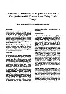
Figure 1. The patternin A is readily interpretedas a parallelogrampartly occludingthe shape in B, rather than the arrow in C. This preferencecould be claimedto occur either because, unlike the shape in B, the arrow would have to take a rather coincidentalposition to obtain the pattern in A or because the shape in B is simplerthan the arrow. Probably,however, both aspects play a role. yet be compared theoretically. Table 1 presents the general framework of this comparison, the details of which are specified in the course of this study. The point is that, in the simplicity-likelihood debate, the actual controversies often seem to have been obscured by the lack of clear distinctions between viewpoint-dependent and viewpointindependent aspects of perception and between probabilistic and descriptive accounts of these two types of aspects. I analyze these distinctions in the historical context of the simplicity and likelihood paradigms, now and again using some reformulations that facilitate a theoretical comparison of the two paradigms. This analysis has been made possible by, among other things, very intriguing findings in the mathematical research area of algorithmic information theory (AIT). For a mathematical introduction to AIT, I refer to Li and Vitfinyi's (1997) book An Introduction to
771
Kolmogorov Complexity and Its Applications, which has been my main guide into AIT. A1T is devoted largely to the question of how simplicity and likelihood are actually related, and fairly recent results in AIT suggest that simplicity and likelihood might well be very close (see also Vitfinyi & Li, 2000). In this study, I elaborate on this insight from AIT to assess how close simplicity and likelihood are in perception. I owe credit to Chater (1996) for drawing attention to AIT, even though his discussion of AIT findings is rather flawed (see the Appendix). Chater wrongly suggested that he settled the question of how close simplicity and likelihood are by claiming to have proved that the simplicity and likelihood principles are formally equivalent. At best, however, his article can be read as a halfhearted rejection of Pomerantz and Kubovy's (1986) proposal to redefine the simplicity principle in terms of the likelihood principle and as an unsupported approval of Leeuwenberg and Boselie's (1988) inverse proposal to redefine the likelihood principle in terms of the simplicity principle. In this study, I use AIT findings to put these two proposals in a new perspective by assessing, for each principle, how such a redefinition relates to its original definition. This article consists of four fairly separate parts and a general discussion. In the relatively long first part, The Simplicity and Likelihood Principles in Perception, I discuss the development of the simplicity and likelihood principles in perception research, and I analyze the distinction between (and subsequent integration of) viewpoint-dependent and viewpoint-independent aspects of perception. In the second part, The Age of Information, I discuss the classical information-theoretic ideas about the relation between simplicity and likelihood, and I sketch how these ideas caused a paradigm shift from probabilistic to descriptive accounts in perception as well as in mathematics. In the third part, Structural Versus Algorithmic Information Theory, I go into more detail on the differences and parallels between perception and AIT to enable a proper appreciation of AIT findings. In the fourth part, The Relation Between Simplicity and Likelihood, I sketch how AIT research has led to deep mathematical insights into the relation between simplicity and likelihood. In the General Discussion, I argue that either principle may have guided the evolution of visual systems because, among other things, the two principles seem to be close with respect to the viewpoint-dependentaspects which are
Table 1 Visual Perception and the Simplicity and Likelihood Principles Visual perception Input Output
Viewer-centered proximal stimulusD Object-centered interpretationH (Hypothesis about what the distal stimulus is) Hypotheses judged on Viewpoint-independenta s p e c t s (distal stimulus as such)
Viewpoint-dependent aspects (relation to proximal stimulus)
Likelihood formalization Simplicityformalization
Prior probabilityp(H) Prior complexityI(H)
Conditionalprobabilityp(D[H) ConditionalcomplexityI(D]I-1)
Resulting interpretation Likelihood principle Simplicityprinciple
The hypothesis H that maximizesp(I~D) = p(H) × p(DIl-1) The hypothesis H that minimizesI(I-~D) = I(H) + I(D[H)
772
van DERHELM
decisive in everyday perception. My overall conclusion is that the simplicity paradigm may provide perception models with the necessary quantitative specifications of the often plausible but also intuitive ideas provided by the likelihood paradigm. The Simplicity and Likelihood Principles in Perception Here, I review the development of the simplicity and likelihood principles in perception research. I focus on historical aspects that are directly relevant to the distinction between viewpoint independencies and viewpoint dependencies (for alternative or broader historical views, see, e.g., Gigerenzer & Murray, 1987; Gordon, 1997; Palmer, 1999; Pomerantz & Kubovy, 1986).
The Likelihood Principle The likelihood principle was initiated about one century ago by von Helmholtz (1909/1962). It states, more specifically than I sketched earlier, that "we perceive the most likely objects or events that would fit the sensory pattern that we are trying to interpret" (Hochberg, 1968, p. 89; for similar formulations, see, e.g., Gregory, 1973, and Pomerantz & Kubovy, 1986). Perception is thus conceived as a neural activity the outcome of which can be modeled by a process of hypothesis testing, eventually selecting the most likely hypothesis. In other words, perception is modeled as selecting, for a given proximal stimulus, the interpretation with the highest probability of being correct, that is, with the highest probability of specifying the really present distal stimulus. Hence, in fact, the likelihood principle corresponds to the assumption that perception is as veridical as it can be. In the following subsections, I review how likelihood approaches have addressed the question of, so to speak, where the perceptual system gets its probabilities from. I first discuss this briefly for viewpoint-independent aspects of perception and then more extensively for viewpoint-dependent aspects. Finally, I discuss how these two types of aspects may be integrated within the likelihood paradigm. Viewpoint-independent aspects and prior probabilities. Traditional ideas, within the likelihood paradigm, are that the probability of an interpretation is higher if the interpretation reflects a situation that occurs more frequently in this world or if it is more familiar or biologically more important as reflected by ontogenetically or phylogenetically acquired knowledge--see, for example, Pomerantz and Kubovy (1986), Gigerenzer and Murray (1987), Gordon (1997), and Palmer (1999) for more extensive discussions of such ideas by, for example, Ames (1949), Brunswick (1956), Hochberg (1968), Neisser (1976), Gregory (1980), and Rock (1983). It is difficult to assess whether the visual system is indeed guided by such real-world probabilities. To my knowledge, such real-world probabilities have never been really determined by, for instance, counting how frequently certain things occur in this world. Besides, what are the categories of things to be distinguished, and how are these categories distinguished? Is one category a specific object, or is it an object set of, for example, all cubes of a specific size, or is it a structure set of, for example, all cubes (disregarding size differences), or is it a property set of, for example, all symmetries in all objects? Despite these questions, i t is yet plausible that visual systems have somehow undergone an evolutionary adaptation to real-world
probabilities.1 Be that as it may, note that these probabilities are typically attributes of distal stimuli. That is, these probabilities are already fixed prior to the actual presence of a proximal stimulus and are thereby independent of the viewpoint position of the perceiver. These viewpoint-independent probabilities are therefore also called prior probabilities. In this study, I refer to the idea of frequencies of occurrence as a pars pro toto for the aforementioned ideas about the real-world origin of these prior probabilities.
Viewpoint-dependent aspects and conditional probabilities. More recent likelihood approaches by, for example, Rock (1983), Pomerantz and Kubovy (1986), Biederman (1987), and Hoffman (1998) proposed heuristics that are useful for inferring likely interpretations from a given proximal stimulus. Many of these heuristics reflect so-called Gestalt laws of perceptual organization. Gestalt psychologists (K6hler, 1920; Wertheimer, 1923) proposed these laws as principles guiding the perceptual grouping of elements in a stimulus. Examples of these grouping principles are proximity, symmetry, similarity, and good continuation. The law of proximity, for instance, expresses that stimulus elements tend to be grouped together if they are relatively close to each other. I refer the reader to Pomerantz and Kubovy (1986) for an extensive discussion of this link between Gestalt psychology and the heuristics as used in the more recent likelihood approaches. My present point is that a lot of these heuristics deal with the viewpoint position of the perceiver. For instance, in the introduction, I alluded to Rock's (1983) avoidance-of-coincidence heuristic, which excludes interpretations that imply an accidental viewpoint position with respect to shapes arranged in depth. In a similar vein, Binford (1981), Witldn and Tenenbaum (1983), and Biederman (1987) argued that a proximal straight line can safely be interpreted as a distal straight edge because it can be caused by a distal curved edge only from an accidental viewpoint position. They therefore referred to straightn e s s - a n d also to, for example, symmetry--by the term nonaccidental property: If such a property is present in the proximal stimulus, then it is most likely also present in the distal stimulus. These ideas reflect the general viewpoint assumption: A proximal stimulus is interpreted assuming it does not contain features that would arise only from an accidental viewpoint position with respect to the distal stimulus. In other words, the probability of the perceiver taking a general viewpoint position is a priori assumed to be high. The general viewpoint assumption is indeed plausible, but it seems better to formulate it in another way. That is, the probability of the perceiver taking a general viewpoint position is not one fixed probability but varies with the distal stimuli at hand. For instance, apart from orthofrontal rotations, a straight needle seems
1 This may also indicate that the likelihood principle is generally understood to imply that perceptual preferences are based on some form of long-term learning, rather than on a form of short-term learning. For instance, within the miniature world of a single experiment, one may first present a number of same and different views of an object and then test whether a subsequently presented view leads to faster recognition if it is closer to a previously more frequently presented view (cf. Tan', 1995). Such short-term learning experiments, however, are about how preferred interpretations, in this case, of the previously presented views, might be represented in memory rather than about the currently relevant issue of how perception selects the interpretations it prefers.
SIMPLICITY VERSUS LIKELIHOOD to give rise to only two nongeneral viewpoint positions (i.e., those yielding a proximal dot), whereas a solid cube seems to give rise to at least six nongeneral viewpoint positions (i.e., those yielding a proximal square). Therefore, it seems better to formulate the general viewpoint assumption in terms of so-called conditional
probabilities: The conditional probability of an interpretation is the probability that the given proximal stimulus arises, conditional on the real distal stimulus being as hypothesized. For instance, a distal straight edge yields proximally a straight line from almost any viewpoint position, so that the hypothesis that a proximal straight line is caused by a distal straight edge has a very high conditional probability. Analogously, the hypothesis that it is caused by a distal curved edge has a very low conditional probability. Conditional probabilities reflect the degree of consistency between a proximal stimulus and each of the candidate distal stimuli. Thereby, conditional probabilities account for viewpointdependent aspects of perception. Furthermore, this analysis shows that the general viewpoint assumption is plausible because it favors interpretations with high conditional probabilities (i.e., rather than because it gives the perceiver a high prior probability of taking a general viewpoint position). In order to give a gist of how conditional probabilities may be determined, I consider the patterns in Figure 2. Each of the six patterns A - F in Figure 2 can be interpreted as a rectangle plus a triangle. Under this interpretation, however, the patterns exhibit different numbers of coincidences in Rock's (1983) sense. For instance, Pattern A exhibits no coincidences, whereas Pattern B
Figure 2. Going from Pattern A to Pattern F, the triangle can intuitively be said to take a more and more coincidental position relative to the rectangle. This intuition presupposes certain categories of relative positions (so that an intuitively more coincidental relative position belongs to a smaller category) because, otherwise, all relative positions would be equally likely.
773
exhibits one coincidence, namely, an edge in the rectangle coincides with a junction of edges in the triangle. Similarly, each of the other patterns, too, can be seen as belonging to a specific coincidence class of relative positions. Assuming a restricted resolution, one may count how many relative positions of the rectangle and the triangle would fall in the same coincidence class. For each pattern and after normalization, this number of relative positions can then be taken as the conditional probability of the rectangle + triangle interpretation. Going from Pattern A to Pattern F, one thus finds that this conditional probability gradually decreases. Of course, analogous to the previous subsection, pending questions here are which coincidence classes are to be distinguished, and how are they distinguished? After all, without presupposing such classes, all relative positions would be equally coincidental-only with such classes, the coincidentality of a relative position can be assessed on the basis of the size of its class (i.e., it is more coincidental if it belongs to a smaller class). Yet, intuitively, this method of determining conditional probabilities seems plausible, and, as a final example, it also implies that the nonpreferred arrow interpretation in Figure 1 has a relatively low conditional probability. Integrating prior and conditional probabilities. The foregoing indicates that the traditional likelihood approaches tended to focus on the viewpoint-independent prior probabilities of interpretations, whereas the more recent likelihood approaches tended to focus on the viewpoint-dependent conditional probabilities of interpretations (see also Gigerenzer & Murray, 1987, who used different wordings to stress the relevance of the same distinction between prior and conditional probabilities). In this subsection, I discuss how Bayes's rule can be used to integrate prior and conditional probabilities, even though the need for such an integration is perhaps not obvious. 21 use Bayes's rule because, on the one hand, the main arguments in this study are at a level that transcends the level of specific models, while on the other hand, the Bayesian integration is open to any desired specification of either component (see also Watanabe, 1969). One might, for instance, choose the prior probabilities to be uniform so that the conditional probabilities become completely decisive (cf. Gigerenzer & Murray, 1987)~ To provide a good insight into the interpJay of prior and conditional probabilities, I first illustrate Bayes's rule by means of a hypothetical AIDS test that seems reliable in that 90% of its results are correct (see Table 2 for the quantitative details). For given data D to be explained, Bayes's rule states that the so-called posterior probability p(HID) of hypothesis H being true is proportional to the prior probability p(H) of H multiplied by the conditional probability p(D[I-1)of D given H. (The proportionality constant, or normalization, is presently 'less relevant--it comprises the probability p(D) that data D occur; see also Table 2.) Now, for
2 To be clear, an integration of prior and conditional probabilities is not in conflict with arguments that mental representations primarily comprise viewpoint-independent aspects (see, e.g., Biederman & Gerhardstein, 1993) nor with opposite arguments that they primarily comprise viewpointdependent aspects (see, e.g., Tarr, 1995). That is, these arguments are about the character of already-stored mental representations (for an integration proposal regarding this memory issue, see Leeuwenberg & van der Helm, 2000), whereas the present issue is about the criterion for the selection of interpretations still to be stored. Such a selection criterion does not prescribe which aspects of a selected interpretation will be stored in memory.
774
VAN DER H E L M
Table 2
Application of Bayes' s Rule to a Hypothetical AIDS Test Bayes's rule
Posterior = (prior × conditional)/normalization
Priors
p(--dlDS) = 98%
Test result is negative (NEG) Conditionals Normalization Posteriors
p(NEGI--~AIDS) = 90% p(NEGIAIDS) = 10% p(--~AIDS) × p(NEGI--ctlDS) + p(AIDS) × p(NEG[AIDS) = 88.4% p(--dlDSINEG) = 99.8% p(AIDSINEG) = 0.2%
Test result is positive (POS) Conditionals Normalization Posteriors
p(POSI--dlDS) = 10% p(POS~41DS) = 90% p(--riDS) × p(POSI--ctlDS) + p(AIDS) × p(POS~41DS)= 11.6% p(--~AIDS[POS) = 84.5% p(AIDSIPOS) = 15.5%
p(AIDS) = 2%
Note. On this hypothetical AIDS test, 90% of AIDS patients score positive, while 90% of the others (--rIDS) score negative, that is, 90% of all test results are correct. In this example, 2% of the entire population has AIDS.
the AIDS test, the 90% correct results specify only the conditional probabilities p(POS~tlDS) and p(NEGI--~41DS), that is, 90% of subjects with AIDS score positive on this test, and 90% of subjects without AIDS score negative. For an individual subject who, for instance, scored positive, however, the question is how reliable this score is--after all, 10% of subjects without AIDS also score positive. The application of Bayes's rule shows that a negative score is indeed very reliable but also that a positive score is actually very unreliable due to the very low prior probability p(AIDS) = 2%. Suppose, for instance, that 1,000 arbitrary participants are to be tested. The prior probabilities imply that, among these 1,000 participants, there will be about 20 (i.e., 2%) with AIDS and about 980 (i.e., 98%) without AIDS. The conditional probabilities then imply that a positive score will result for about 18 (i.e., 90%) of the 20 participants with AIDS and for about 98 (i.e., 10%) of the 980 participants without AIDS. This means that by far, most of the positive scores, namely, 98 out of 116, will be false alarms, which corresponds to the Bayesian posterior probability p(--dlDSIPOS) = 84.5%. The foregoing example shows that Bayes's rule provides an appropriate account of the interplay of prior and conditional probabilities. In perception, Bayes's rule can be used to characterize the likelihood principle as stating that the visual system, when presented with a proximal stimulus D, selects the interpretation H that maximizes (the normalization can now be omitted)
p(nlD) = p(H) X p(Oln).
(1)
Hence, here, p(H) is the viewpoint-independent prior probability of interpretation H, whereas p(DIH) is the viewpoint-dependent conditional probability that proximal stimulus D arises if the distal stimulus is as hypothesized in interpretation H. The combination then yields the inferred posterior probability p(l~D) that H specifies the really present distal stimulus. For instance, reconsider the heuristic that a proximal straight line is caused by a distal straight edge rather than by a distal curved edge. Pomerantz and Kubovy (1986, p. 13) argued that this heuristic should be justified by showing that, in this world, straight edges occur more frequently than curved edges (they also remarked that it remains to be seen whether this world complies with this requirement). This would be a justification in terms of prior probabilities only, whereas the heuristic actually derives its plau-
sibility largely from the fact that the straight edge hypothesis has a high conditional probability (see previous subsection). Yet, in a sense, Pomerantz and Kubovy were correct because, as illustrated above for the AIDS test, a high conditional probability may well be suppressed by a low prior probability. That is, in the case of the straight edge hypothesis, the conditional probability is perhaps high, but this hardly affects Pomerantz and Kubovy's remark that it remains to be seen whether the prior probability is high enough to allow a probabilistic justification of the heuristic (Leeuwenberg et ai., 1994). The foregoing shows that the likelihood paradigm gives rise to an intuitively plausible model for the integration of viewpointindependent and viewpoint-dependent aspects of perception. Yet two modeling questions remain pending. First, for both types of aspects, it is as yet unclear how to distinguish between the categories to which probabilities are to be assigned. Second, without an actual quantification of the prior probabilities (if not taken to be uniform), it seems hardly possible to perform a critical test of the likelihood principle. Now, the remainder of this article shows, in fact, how the simplicity paradigm might provide answers to these questions. First, in the next section, I show that the simplicity paradigm gives rise to an alternative model for the integration of viewpoint-independent and viewpoint-dependent aspects.
The Simplicity Principle In the previous section, I mentioned that the early 20th century Gestalt psychology influenced later developments within the likelihood paradigm. Gestalt psychology led, however, also to the simplicity principle, as follows. Koffka (1935/1962) concluded that there might be one general principle underlying all of the Gestalt laws, and he called this principle the law of Pragnanz. Although the meaning of the German word Prtignanz is rather fuzzy (see Arnheim, 1987), it is generally understood to imply something like a tendency towards stability, harmony, and simplicity. One might also understand it to imply that perception is conceived as a neural system that, when presented with a stimulus, exhibits the tendency of many other physical systems, that is, the tendency to settle into an equilibrium involving minimum energy load. The resulting neural pattern of activation then forms the mental representation of the stimulus interpretation. Be that as it
SIMPLICITY VERSUS LIKELIHOOD may, Koffka's idea, combined with developments in classical information theory (see the second part of this article, The Age of Information), led Hochberg and McAlister (1953) to propose the simplicity principle, as follows: the less the amount of information needed to define a given organization as compared to the other alternatives, the more likely that the figure will be so perceived. (p. 361) (Hochberg & McAlister called it the minimum principle to indicate that perception tends to minimize information loads, in analogy to the tendency of physical systems to minimize energy loads.) At the same page, they specified information loads further, by the number of different items we must be given, in order to specify or reproduce a given pattern. (p. 361) This means, in other words, that perception is modeled as selecting the most simple interpretation of a given stimulus, where the complexity of an interpretation is defined by the amount of socalled descriptive information needed to specify the interpretation such that the stimulus can be reproduced (see also Attneave, 1954, for an early theoretical discussion of this idea). 3 The simplicity principle can perhaps be seen as just another alternative within the likelihood paradigm, given that it can be conceived as stating that the probability of an interpretation is higher if the interpretation is simpler. Then, however, a crucial difference still would be that the likelihood principle, as it stands, can be said to infer the probability of an interpretation from an analysis of the world, whereas the simplicity principle infers this probability from an analysis of the interpretation itself. These options reflect different answers to the earlier mentioned question of, so to speak, where the perceptual system gets its probabilities from. In this respect, the simplicity principle pretends to be an alternative to the likelihood principle, rather than an alternative within the likelihood paradigm. Yet, either way, it raises the question of how the simplicity principle's probabilities would relate to the likelihood principle's probabilities. This question is addressed extensively in the fourth part, below, The Relation Between Simplicity and Likelihood. Until then, I focus on Hochberg and McAlister's (1953) basic idea that simplest descriptions might be used to predict stimulus interpretations. During the past 4 decades, this idea has been implemented in various so-called perceptual coding languages (see, e.g., Dastani, 1998; Feldman, 1997; Leeuwenberg, 1969, 1971; Restle, 1970, 1979, 1982; Simon & Kotovsky, 1963; Vitz & Todd, 1969). Such a perceptual coding language is in fact a descriptive coding language, that is, it can be used to describe any arbitrary stimulus. Which specific stimulus descriptions (i.e., stimulus interpretations) are possible depends on which specific coding language is chos e n - t h i s issue is addressed in the third part, Structural Versus Algorithmic Information Theory. Here, I focus on the use of descriptive coding languages in general. Basically, a coding language is a scientist's tool for obtaining complexities--just as, within the likelihood paradigm, counting would be a method of obtaining probabilities in terms of frequencies of occurrence. However, coding languages also incorporate much of the philosophy behind the simplicity paradigm. Therefore, in the next subsection, I elaborate on the character and potential relevance of descriptive coding languages (without singling out a
775
specific coding language), and I discuss mathematical and psychological evidence that complexities are fairly independent of the chosen coding language. After that, I discuss how, within the simplicity paradigm, viewpoint-independent and- viewpointdependent aspects of perception have been dealt with.
Descriptive coding languages and the lnvariance Theorem. Probably not by chance, the first perceptual coding languages were developed in the early days of the computer age. Indeed, as I assess first, perceptual coding languages have a lot in common with computer programming languages such as FORTRAN and PASCAL. A computer programming language comprises a set of instruction rules enabling a programmer to compile a code that, when run on a computer, produces certain output. In other words, the computer code represents a way to obtain this output. For instance, in order to produce the letter sequence ababab.., abab consisting of, say, 600 letters, one could execute a computer code like for i = 1 to 150 do { print(a), print(b), print(a), print(b) } or, alternatively, a computer code like for i = 1 to 300 do { print(a), print(b) }. Similarly, a perceptual coding language comprises a set of coding rules enabling the compilation of a code that represents a way to construct a certain pattern. For instance, for a parallelogram with sidesy = 5 cm, z = 3 cm, and angles a = 70 ° , /3 = 110% a perceptual code could be something like 2 * (yotz/3). This code can be seen as an instruction to be executed by a plotter, in which case it would yield a drawing of the parallelogram. If it so happens that, for example, y = z = 3 cm and tx = / 3 = 90 °, this same code 2 * (yotz/3) would produce a square--then, an alternative code is of course also something like 4 * (yot). Thus, basically, both computer codes and perceptual codes are so-called descriptive codes, that is, codes that constitute reconstruction recipes. Another common characteristic of computer codes and perceptual codes is their so-called hierarchical structure (see also Simon, 1972). For instance, the two computer codes given above for the letter sequence ababab.., abab reflect descriptions at the level of letters. However, so that, for example, a laser printer can put the letter a on paper (as instructed by the statement "print(a)"), somewhere down the line the laser printer has to be fed with a description of the letter a at the level of laser-printer pixels. Similarly, a perceptual code of the pattern '.. ".. '.. '.. "-. ".. could comprise a description like 6 * (t) at the level of dot-triples but only if t refers to a description like 3 * (d) at the level of dots, in which, in turn, d refers to a description of a dot at the level of, say, perceptual pixels. Thus, a descriptive code comprises in fact a hierarchy of description levels in which, recursively, each level involves a description that builds on its lower levels.
3 The simplicity principle has sometimes been associated with simplicity in terms of the processing efficiency (regarding, e.g., speed or number of steps) or the hardware reliability of the visual system (cf. Hatfield & Epstein, 1985). This kind of simplicity is perhaps relevant but is not considered in this study. Instead, I consider Hochberg and McAlister's (1953) kind of simplicity, which, just as likelihood, applies to the outcomes of the visual process. In the fourth part, The Relation Between Simplicity and Likelihood, the latter kind of simplicity is discussed in terms of efficiency and reliability but, then, regarding the required short-term memory capacity and the real-world veridicality of predictions, respectively.
776
VANDERHELM
T h e foregoing implies that different descriptive codes of one and the same object (i.e., certain computer output or a visual pattern) may specify, for this object, different classifications and different hierarchical organizations (see also Figure 3). For instance, as indicated, the perceptual codes 4 * (ya) and 2 * (yaz/3) both may produce the same square, that is, when supplied with the proper numerical values of the symbols. Then, in fact, the former code specifies a quadrangle consisting of four identical sides and four identical angles (which can be nothing but a square), whereas the latter code specifies a quadrangle in which opposite sides and angles are identical (which is the definition of a parallelogram). In other words, the former code classifies the square as square, whereas the latter code classifies the square as parallelogram. Furthermore, for the letter sequence ababab.., abab, the first computer code above describes the sequence as having a hierarchical organization consisting of 150 chunks abab, whereas the second computer code above describes it as having a hierarchical organization consisting of 300 chunks ab. In the theory of computer languages, classification and hierarchy do not seem to be major issues as such, that is, they seem to be conceived primarily as means to obtain compact codes of objects. In the theory of perceptual languages, however, classification and hierarchy are considered to have an intrinsic relevance, too, in that they might reflect the categories that play a role in perception. The classification issue is discussed more extensively in the third part, Structural Versus Algorithmic Information Theory. Here, it seems expedient to go into some more detail on three aspects of the hierarchy issue. First, the hierarchical structure of descriptive codes allows for the simultaneous description of different features not only at a same hierarchical level but also at different hierarchical levels. In the latter case, the features are related asymmetrically. For instance, a circular pattern built up from small squares exhibits a hierarchy of the features circle and square, which is the inverse of the hierarchy exhibited by a square pattern built up from small circles (see also Leenwenberg & van der Helm, 1991). The hierarchical structure of descriptive codes might well be helpful in solving the classical Gestalt problem of how to capture the interplay of competing Gestalt laws in a given pattern: Gestalt laws
/? Figure 3. The pattern in A can be described in various ways, each description reflecting another organizationof the pattern. It can, for instance, be described and organized as consistingof two triangles(B), two diabolos (C), or two parallelograms(D). (After Reed, 1974.)
apply to separate features, but simultaneouslypresent features may have different effects in different patterns. Some of these differential effects might be captured by the asymmetry between hierarchical levels in descriptive codes (cf. Neisser, 1967). Second, Pascal (1658/1950) observed that a description hierarchy seems to comprise a n infinite number of semantically related nominalistic levels of description. That is, each hierarchical level contains symbols which are meaningful only in relation to the lower levels which describe what these symbols stand for. This holds of course also for the lower levels, so that the total number of levels seems to be infinite--at least, it is unclear what the lowest level might be. In computer theory, this problem has been solved by taking as the lowest level the level of binary sequences into which any higher level instruction is translated before it is executed. In perception theory, Pascal's problem reappears as the so far unsolved question of what the so-called perceptual primitives are: Are they pixels, dots, edges, blobs, or what? Biederman (1987), for instance, proposed to solve this question by using a restricted set of prechosen primitives called geons (simple volumetric building blocks). Pragmatically, this is perhaps a convenient solution, but, theoretically, it is not very satisfactory (Kurbat, 1994; Leeuwenberg et al., 1994). Within the simplicity paradigm, the idea is that perception starts with considering all possible primitives and that those leading to the simplest descriptive code will be the perceptual primitives for the stimulus at hand (see also Palmer & Rock, 1994, for a similar fluid notion of primitives). Third, in practice, users of a descriptive coding language generally work with only the highest levels in the description hierarchy, meaning that the topic under investigation is assumed to be tractable without having to bother about lower level details. The choice to start the encoding at some level is not a choice between languages (as suggested by, e.g., Chater, 1996), but it is a choice within a language. If, for instance, perceptual research on dot patterns is at hand, then it may be reasonable to work with codes starting at the level of the dots--unless, for example, the dots have varying shapes or colors, in which case one may have to start at a lower level to get a proper account of the perceptual variation within the stimulus set at hand. In other words, it seems reasonable to start the encoding at the level just below the level at which the stimuli start to show distinctive properties. Similar considerations apply to the practice of computer programming: Usually, it suffices to program in terms of higher level instructions, without having to bother about how these instructions are implemented at lower levels. Now, the entire simplicity paradigm actually leans on the fact that different descriptive codes of the same object not only specify different classifications and organizations but, generally, also have different lengths (with, as may be clear, a special status for the shortest one). This, too, is illustrated by the two computer codes for the letter sequence ababab.., abab and by the two perceptual codes for a square (assuming that these highest description levels are representative for the entire description hierarchy). These examples also illustrate that the length of a descriptive code depends on the amount of regularity accounted for (see also Simon, 1972). That is, in general, shorter descriptive codes of an object are obtained by "squeezing out" more regularity. Thus, descriptive coding languages establish a link between what Hatfield and Epstein (1985) called descriptive simplicity (in terms of code compactness) and phenomenal simplicity (in terms of regularity).
SIMPLICITY VERSUS LIKELIHOOD There is much more to say about descriptive code lengths (see the third and fourth parts, below), but for the moment, it may suffice to note that these lengths correspond quite well to Hochberg and McAlister's (1953) notion of complexity as being "the number of items we must be given" (p. 361). The foregoing suggests that the simplicity paradigm can be seen as a scientific enterprise that, at one stroke, might solve the two questions that remained pending for the likelihood paradigm. That is, first, descriptive codes might specify the perceptual categories to which probabilities are to be assigned, and, second, the complexities of these codes might be used to quantify these probabilities. Thus, the simplicity paradigm might provide a quantitative specification of the intuitive notions provided by the likelihood paradigm. This is the enterprise Hochberg and McAlister (1953) more or less proposed and that has been explicitly promoted by Leeuwenberg and Boselie (1988). By the way, once the perceptual categories have been specified by means of descriptive codes, one could of course still decide to search for their real-world probabilities. However, descriptive codes, regularity, and simplicity form a strong trinity, so that it seems expedient to at least consider the option of using complexities to quantify probabilities. This option might be fruitful especially in situations like perception where one does not have direct access to the real probabilities. In mathematics, Solomonoff (1964a, 1964b) explicitly had such situations in mind when he proposed to undertake the very same scientific enterprise (see the fourth part, The Relation Between Simplicity and Likelihood). Solomonoff (1964a, 1964b) not only was interested in the possibility of a useful relation between complexities and probabilities (rather than in the categorization issue) but also solved a problem that seemed to nip the entire enterprise in the bud. That is, if one defines the complexity of an object by the length of its shortest description, then different descriptive coding languages generally yield different complexities for one and the same object. Hence, it seems impossible to speak of "the" complexity of an object. Thus, the question is: Which descriptive coding language should be used? Solomonoff, however, showed that it does not matter much which descriptive coding language is used because the complexity of an object cannot vary arbitrarily over descriptive coding languages. More formally, two languages L 1 and L 2 may yield different complexities Cl(x) and C2(x) for the same object x, but Solomonoff (1964a, 1964b) proved that the absolute difference IC2(x) Cl(x) I is smaller than some constant that depends on only the two languages (i.e., not on the object). To give a gist in terms of computer languages, let Cr. P be the length of the shortest PASCAL code that translates any FORTRAN code into its equivalent in PASCAL, and let x be the output to be produced. Now, if CF(X) is the length of a shortest FORTRAN code of x, then one can write a PASCAL code that consists of this shortest FORTRAN code of size CF(X)plus the translator code of size CF.P. This PASCAL code first translates the FORTRAN code into PASCAL and then executes this translation to produce x. Often, there will be even shorter PASCAL codes for producing x, so, in general, the complexity Cp(x) in PASCAL will be smaller than or equal to CF(X) + CF.p, in which the constant Cr. r, depends on only the two languages. One may still debate the precise size of the constant, but, in general, Solomonoff's finding implies that different descriptive coding languages yield object complexities that are fairly close to one
777
another. In other words, it implies that simplicity is a fairly stable concept and that, to a high degree, it is yet possible to speak of "the" complexity of an object. Solomonoff's fmding, known as the lnvariance Theorem, marked the beginning of AIT as a separate mathematical research area. Independently, this theorem has been proved too by the other two founding fathers of AIT, Kolmogorov (1965) and Chaitin (1969). Also independently, Simon (1972) observed this invaria n c e in perception. Simon compared six perceptual coding languages from the literature and found that their quantifications of complexity are highly correlated. Simon's finding can be seen as an empirical proof that the Invariance Theorem is valid in perception. Simon also remarked, however, that this invariance does not pertain to the categorization issue, that is, different sets of coding rules yield different categories. Hence, a psychological foundation of the employed coding rules remains necessary (for this, see the third part, Structural Versus Algorithmic Information Theory). The foregoing shows that, at least regarding the quantification of complexity, it does not seem to matter much which perceptual coding language one chooses to use. Therefore, in this study, I choose one perceptual coding language as a pars pro toto, namely, Leeuwenberg's (1969, 1971) coding model which became known as the structural information theory (SIT). An obvious reason for me to choose SIT is my own involvement in the SIT research group at the University of Nijmegen--but there is more to say about this choice. SIT has faced several problems regarding, for instance, the choice of its coding rules and its complexity measurement and the computability of its simplest codes--see, for example, Simon (1972), Collard and Buffart (1983), Hatfield and Epstein (1985), and Pomerantz and Kubovy (1986). These problems, however, have largely been overcome (see also the third part, below). Despite various remaining problems (which keep the research group going), SIT is nowadays probably the most elaborated coding approach in perception (as this study may be proof of; see also, e.g., Palmer, 1999). Analogous to the earlier discussed likelihood approaches, SIT conceives perception as a neural activity the outcome of which can be modeled by a process of hypotheses testing--but now selecting the most simple hypothesis. Also analogously, SIT started out focusing primarily on viewpoint-independent aspects of perception. Later, SIT began considering viewpoint-dependent aspects, albeit actually to argue that these aspects are subordinate to viewpoint-independent aspects (Buffart, Leeuwenberg, & Restle, 1983; Leeuwenberg & Boselie, 1988; Leeuwenberg et al., 1994). More recently, however, SIT has included viewpoint-dependent aspects as a separate factor that is to be integrated with viewpointindependent aspects (van Lier, van der Helm, & Leeuwenberg, 1994, 1995). This integrative approach is discussed next.
Viewpoint-independent aspects and prior complexities.
Anal-
ogous to the notion of prior probability, one may define the prior complexity of a stimulus interpretation as the complexity of the distal shapes as hypothesized in this interpretation, independent of the actual proximal stimulus: Thus, as before, this complexity is already fixed prior to the actual presence of a proximal stimulus and is thereby independent of the viewpoint position of the perceiver. For instance, Figures 1B and 1C depict two interpretations of the pattern in Figure 1A, each interpretation specifying a distal shape that is hypothesized to be the one that is partly occluded by the parallelogram. The prior complexity of each interpretation then
778
VANDER HELM
amounts to the sum of the complexity of the parallelogram and the complexity of this hypothesized shape. Because the shape in Figure 1B has a simpler code than the arrow in Figure 1C, its corresponding interpretation has a lower prior complexity. Similarly, for a proximal straight line, the straight edge hypothesis has a lower prior complexity than the curved edge hypothesis. This picture of prior complexities touches two currently relevant issues. First, it could be argued that a simple form is, in an evolutionary sense, more prone to leave a strong neural trace because, for example, it can be stored succinctly and retrieved quickly, which could imply a high prior probability. This argument might even fit in the likelihood paradigm (cf. Pomerantz & Kubovy, 1986, p. 10). However, as indicated earlier, this study is meant to assess whether the simplicity paradigm might be an alternative to, rather than within, the likelihood paradigm. Now, in the likelihood paradigm, prior probabilities are based on, for example, frequencies of occurrence in this world, and there seems to be no reason to assume that these might somehow correspond quantitatively to prior complexities. This can be seen as an indication that the simplicity and likelihood principles are not particularly close--at least not with respect to the viewpoint-independent aspects of perception. Second, within the likelihood paradigm, an explicit specification of the perceptually relevant categories has to precede the determination of the prior probability for an individual case. In contrast, as discussed by Collard and Buffart (1983), within the simplicity paradigm, each descriptive code implicitly induces a category (in the spirit of Garner's [1962] so-called inferred subsets; see the third part, Structural Versus Algorithmic Information Theory). For instance, the simplest code of a specific square implicitly induces the category of all possible squares. Thus, now, the categories in fact succeed the determination of the prior complexity for an individual case. This suggests that the order of determination might be as follows: first the prior complexity, then the category, and only then the prior probability. Be that as it may, the foregoing indicates that the categories might well be crucial in assessing how close prior complexities and prior probabilities are (see the third and fourth parts, below). Viewpoint-dependent aspects and conditional complexities. In the previous section, I discussed how viewpoint-dependent aspects are dealt with, in an intuitively plausible way, by the general viewpoint assumption. I argued that, within the likelihood paradigm, the general viewpoint assumption is best formalized in terms of conditional probabilities, although, even then, there is still the problem of distinguishing between the categories to which these probabilities are to be assigned. Within the simplicity paradigm, however, the general viewpoint assumption can be formalized without the need for explicit a priori categories. This has been shown by van Lier (van Lier et al., 1994), whose line of reasoning I sketch next. Van Lier argued that coincidences, in the sense of Rock (1983), are in fact regularities in the relative position of the shapes in an interpretation (see, e.g., Figure 2). Regularity constitutes a perceptual binding force, that is, in this case, proximally coinciding pattern elements tend to be glued together perceptually (this looks like a genuine Gestaltlike grouping principle). This perceptual glue, however, may contrast with an interpretation in which these pattern elements are specified as belonging to different objects. Therefore, van Lier argued, the effort needed to perceptually dissociate such coincidentally glued elements in fact reflects the
complexity of the relative position of the hypothesized objects in the proximal stimulus. Inversely, one could say that this complexity corresponds to the effort needed to bring the hypothesized objects in their proximal position, starting from a general position of these objects (i.e., a position for which the perceiver can be said to be in a general viewpoint position). The way in which van Lier quantified this complexity, which he called Ioxtern,d, may be illustrated by means of the four patterns in Figure 4. Each of these four patterns can be interpreted as a configuration consisting of one long line segment plus one short line segment (like two sticks thrown on the floor). Figure 4A depicts the two segments in a general, that is, dissociated, position, whereas the other three patterns depict proximal positions in which the two segments are perceptually glued together. Now, van Lier first used SIT's coding model to specify the complexity of each of the four patterns when described as consisting of two segments (see Figure 4). Then, for each of the three proximal positions, he quantified its Iext~ma1 by the complexity difference between the general position and the proximal position (see Figure 4). In line with this, if the proximal position happens to be the general position, it gets an l~xt~m~a = 0 (see Figure 4A). Going from left to right in Figure 4, one thus finds a gradual increase of the l~xt~r~~ for the two segments interpretation. Van Lier also generalized this idea to quantify the complexity of the relative position of twodimensional shapes as hypothesized in interpretations of twodimensional occlusion patterns like the pattern in Figure 1A. For details about this generalization, I refer to van Lier et al. (1994), but just to give a gist: In Figure 2, it implies that, going from Pattern A to Pattern F, one finds a gradual increase of the lext~m~ for the rectangle + triangle interpretation. As a final example, it implies that, in Figure 1, the nonpreferred arrow interpretation has a relatively high Iext~mal'
/ ,/ p ecv 13 q
Ipo~ern
=5
'p-w
iA i s y q
Ipattern
=4
lexternal = 0
lexternal = 1
A
B
pG q
IpaUern
=3
Iexternal = 2 C
p q
I p a t t enr
=2
Iexternal = 3 D
Figure 4. The top row depicts two line segments of lengths p and q in a few relative positions (in B, C, and D, the circle indicates where the segments touch). The middle row depicts how each pattern can be described as consisting of two segments, by a code that comprises a series of line lengths and angles. The number of code elements is taken to quantify the complexity Ipatt~m of the pattern. The complexity l~,aem~ of each relative position is quantified by the difference between the complexity Ip~tt~m of the general situation (in A), and the complexity Ipatt~ of the proximal situation (in A, B, C, or D). (After van Lier et al., 1994.)
SIMPLICITY VERSUS LIKELIHOOD The foregoing indicates that an Iext~m~a value is related to one specific interpretation of a given stimulus, that is, other interpretations of this stimulus generally have different lext~m~a values. In fact, because Iext=.=~a quantifies the difference between proximal and general positions, it can be seen as measuring the degree of consistency between a given proximal stimulus and each of the candidate distal stimuli. In other words, l~xter~ accounts for viewpoint-dependent aspects (van Lier, 1999). In analogy to the notion of conditional probability, I therefore refer to the l~xt~m~aof a hypothesis as the conditional complexity of this hypothesis.4 Furthermore, one may have noticed already that the patterns in both Figure 2 and Figure 4 show a gradual increase not only of the conditional complexity but also of the number of coincidences (in Rock's [1983] sense) that one might count intuitively. In other words, the conditional complexity of a hypothesis seems to be inversely correlated to its intuitively estimated conditional probability. This can be seen as an indication that the simplicity and likelihood principles might be close--at least with respect to the viewpoint-dependent aspects of perception. Finally, van Lier determined conditional complexities without specifying position categories (at the most, perhaps only something like a general viewpoint category). This may indicate that what I stated about the categorization issue in relation to the prior complexities (see previous subsection) pertains just as well to the conditional complexities (see also the third part, below). Integrating prior and conditional complexities. Buffart et al.'s (1981, 1983) attempt, within SIT, to show that the proximal positions of hypothesized shapes are relevant only in the case of otherwise ambiguous patterns turned out to be unsatisfactory (see, e.g., Boselie, 1988; Boselie & Wouterlood, 1989; Kanizsa, 1985; Kanizsa & Gerbino, 1982). Van Lier et al. (1994), however, realized that the viewpoint-dependent conditional complexity of an interpretation can and should be included as a factor separate from its viewpoint-independent prior complexity. They chose to hategrate prior and conditional complexities by simply summing them (see also van Lier, 2000) because this turned out to be sufficient to explain 95% of empirical data they gathered from the literature (most of which contradicted earlier SIT predictions). This integration proposal was developed independently of what turned out to be a parallel proposal in AIT. That is, strengthened by several intriguing AIT findings (see the fourth part, below), Rissanen (1978) proposed the minimum description length (MDL) principle: The best hypothesis to explain given data is the one that minimizes the sum of (a) the information needed to describe the hypothesis; and (b) the information needed to describe the data with the help of the hypothesis. Hence, in this definition, the first amount of information is the prior complexity (given by the shortest description of the hypothesis as such), and the second amount of information is the conditional complexity (given by the shortest description of the data, starting from the hypothesis). Various incarnations of the MDL principle are nowadays being used for prediction in a wide range of statistical problems, among others in molecular biology (see Li & Vit~ayi, 1997, p. 376) and cognitive science (see, e.g., Myung, 2000; Myung & Pitt, 1997). The MDL principle can in fact be seen as a modern version of
779
Occam's razor: A description of raw data as such explains nothing, and it is better to search for some underlying hypothesis by means of which the data can be described more succinctly. The best hypothesis then is as specified by the MDL principle. This Occamian reasoning, by the way, also indicates that a simple summarion of prior and conditional complexities is the proper way to integrate them, just as Bayes showed that a simple multiplication is the proper way to integrate prior and conditional probabilities. The MDL principle in AIT complies with van Lier et al.'s (1994) integrative approach in perception. It gives a formal characterization of the simplicity principle as stating that the visual system, when presented with a proximal stimulus D, seiects the interpretation H that minimizes
I(HID) = I(H) + I(DIH).
(2)
Hence, here, I(HID) is the so-called posterior complexity of interpretation H given proximal stimulus D. This complexity is given by the sum of the viewpoint-independent prior complexity I(H) of the distal shapes as hypothesized in H and the viewpointdependent conditional complexity I(DIH) of proximal stimulus D starting from these hypothesized distal shapes. A few examples may illustrate that perceptual preferences indeed seem to be determined by an integrated interplay of the viewpoint-independent prior complexities and the viewpointdependent conditional complexities. First, in Figure 1, the prior and conditional complexities converge in the sense that they both lead to the more simple shape in Figure IB being preferred over the more coincidental arrow in Figure 1C. Second, relative to the pattern in Figure 5B, the pattern in Figure 5A is more prone to be interpreted as a rectangle partly occluding a simple octagon. In Figure 5B, a more complex shape tends to be preferred because the octagon would have to take a coincidental position which implies a high conditional complexity.
Discussion On the one hand, it is indeed likely that perception is guided by both viewpoint-independent and viewpoint-dependent aspects. On the other hand, it is rather unlikely that the neural perception process explicitly uses either complexities or probabilities to process these aspects. In this sense, the perceptual simplicity and likelihood principles are only suited to model the outcome of the neural perception process, which itself remains what I would call "automagic" (i.e., automatic in some still mysterious way). Indeed, both principles conceive perception as a neural activity the outcome of which can be modeled by a process of hypotheses testing, eventually selecting the most simple or most likely hypothesis. This of course raises the questions of how perception might generate the hypotheses to be tested and how perception might be 41 will not elaborate on the fact that there may be additional viewpointdependent aspects to be accounted for. In occlusion patterns, such an aspect is, for instance, the degree to which a shape is occluded. This aspect seems especially relevant in the case of self-occlusion of three-dimensional objects, for which van Lier currently generalizes his ideas. In his twodimensional occlusion study, van Lier accounted for this aspect by quantifying the complexity of only the occluded part--the sum of this complexity and I,,~t~-~athen forms the total conditional complexity.
780
VANDERHELM
Figure 5. Both patterns are readily interpreted as a rectangle partly occluding another shape. In both patterns, this occluded shape could be an octagon. This octagon interpretation, however, is stronger in Pattern A than in Pattern B because, in Pattern B, the octagon would have to take a rather coincidental position. Therefore, in Pattern B, the occluded shape is more readily taken to be a more complex shape. From "Competing global and local completions in visual occlusion," by R. J. van Lier, P. A. van der Helm, and E. L. J. Leeuwenberg, 1995, Journal of Experimental Psychology: Human Perception and Performance, 21, p. 580. Copyright 1995 by the American Psychological Association. Adapted by permission of the author. (After Kanizsa, 1985.)
able to select a most simple or most likely hypothesis, given the fact that the total number of possible hypotheses is virtually infinite. These questions are, as such, the subject of so-called process models of perception, but, here, it seems useful to indicate briefly some links from the simplicity and likelihood paradigms to process models (see also the third part, below). First, SIT has been linked to connectionistic network models (van der Helm, 1994; van der Vegt, Buffart, & van Leeuwen, 1989) and to models for the detection of visual regularities (van der Helm & Leeuwenberg, 1999). Second, computer vision research uses various incarnations of the heuristics as focused on in the present-day likelihood approaches (see, e.g., Barrow & Tenenbaum, 1986). Indeed, these heuristics can be very useful in generating likely interpretations. For instance, in Figure 1A, the grey edges collide proximally at two places with a straight black edge; such so-called T junctions give a heuristic indication that the grey edges might belong to a partly occluded grey surface. The occluded part then would follow from the heuristic that a proximal straight edge is most likely caused by a distal straight edge plus the heuristic that a partly occluded edge that is straight as far as visible is likely to be straight too as far as not visible. This would imply, in Figure 1A, that the two visible grey edges are continued (behind the occluder) as straight edges until they meet, yielding the shape in Figure 1B (if they would not meet behind the occluder, then additional heuristics might be required). Because, on the one hand, many of these heuristics deal with viewpoint dependencies, while on the other hand, conditional probabilities and complexities seem to be close, it is not surprising that many of these heuristics also fit in the simplicity paradigm, as follows. In general, interpretations with low conditional complexity are, for instance, those which, in line with the general viewpoint assumption, hypothesize that proximal stimulus properties are also present in the distal scene--then, no conditional effort is needed to describe these proximal structures. Furthermore, interpretations with low prior complexity are, for instance, those which extrapolate visible regularity to nonvisible parts (a form of good continuation; see also van Lier et al., 1995). Often, one might thus very well end up with three-dimensional shapes comparable to what one
would get when starting from Biederman's (1987) a priori fixed building blocks called geons. In this sense, Biederman's geon model would fit just as well within the simplicity paradigm as within the likelihood paradigm (Leeuwenberg et al., 1994)--the more because the likelihood paradigm, as it stands, hardly gives rise to heuristics leading to interpretations with a high prior realworld probability (i.e., with, e.g., a high frequency of occurrence in this world). The latter issue touches what seems to reflect a fundamental difference between the simplicity and likelihood principles, namely, the specification of the part of cognition that either principle calls perception. For an extensive discussion of this issue, see Pylyshyn (1999); here, I merely sketch the nature of this difference between the two principles as follows. The priors (i.e., the viewpoint-independent aspects) are, in the likelihood paradigm, judged on the basis of some sort of (generally phylogenetic) knowledge, whereas, in the simplicity paradigm, they are judged independently of knowledge. Thus, the likelihood principle conceives perception as a nonmodular process that is open to influences from already stored knowledge. In contrast, the simplicity principle conceives perception as a modular process, the input of which is solely the proximal stimulus, and the output of which is taken over by higher cognitive processes to be enriched by means of already stored knowledge. This means that, with respect to the priors, there is little hope for a rapprochement of the two principles (even if, as has been proposed within the likelihood paradigm, the prior probabilities would be taken to be uniform). With respect to the conditionals (i.e., the viewpoint-dependent aspects), there seems to be more hope for a rapprochement of the two principles. This can perhaps be understood, rather intuitively, as follows. In the simplicity paradigm, priors and conditionals are determined within the miniature world of a single stimulus. In the likelihood paradigm, conditionals are determined also within this miniature world, but priors are determined within the real world. Compared with the real world, the miniature world gives less room for quantitatively different options. This seems to imply that conditional complexities and probabilities cannot be as different from each other as can prior complexities and probabilities. Stated in a mixture of simplicity and likelihood terms, it might also imply that the real-worid probabilities could well be forming a rather complex probability distribution, whereas the miniature world probabilities are more prone to forming a rather simple probability distribution. In the fourth part, The Relation Between Simplicity and Likelihood, this intuitive argument is formulated in solid mathematical terms. The latter remark already indicates that the remainder of this study is meant to provide further insight into the relation between the simplicity and likelihood principles but in a more formal way. That is, in this first part, I have used specific simplicity and likelihood models to illustrate the underlying ideas which, however, may sometimes still be obscured by the fact that such models will probably always be disputable. Therefore, in the remainder of this study, I investigate the perceptual simplicity-likelihood controversy at a more abstract level. That is, the likelihood principle is taken to start from probabilities given by some, not further specified, probability distribution, while the simplicity principle is taken to start from complexities obtained by means of some, not further specified, descriptive coding language. Furthermore, unless
SIMPLICITY VERSUS LIKELIHOOD stated otherwise, the arguments apply to priors as well as, separately, to conditionals. In order to give a gist of the line of reasoning in the remainder of this study, I conclude this part with a comparison of the two principles as formalized in Equations 1 and 2: Likelihood principle: Select the H that maximizes p(I~D) = p(H) × p(DlI-1). Simplicity principle: Select the n that minimizes I(I~D) = 1(1-1)+ I(DIH). Considering just these formulas, one may observe that, by substituting I = -log2(p) for both the prior and conditional complexities, the simplicity principle becomes equivalent to the likelihood principle. Inversely, by substitutingp = 2 - i for both the prior and conditional probabilities, the likelihood principle becomes equivalent to the simplicity principle. The former substitution complies with Pomerantz and Kubovy's (1986, p. 43) proposal to start from real-world probabilities p and to redefine the simplicity principle such that it uses codes the lengths of which are equal to the so-called surprisal I = -log2(p). The latter substitution complies with Leeuwenberg and Boselie's (1988) inverse proposal to start from descriptive-code complexities I and to redefine the likelihood principle such that it uses probabilities the size of what I call the precisal p = 2 -I. The proposals did not explicitly contain these formulas, but these formulas do express accurately what the proposals amount to. Furthermore, the terms surprisal and precisal are perhaps funny but, for the moment, also convenient references to those formulas--the concepts underlying these terms are explicated in the second and third parts, below, respectively. Chater (1996) mistook each of these equivalence-rendering redefinitions for a proof of the equivalence of the two principles as defined originally (see the Appendix). In Chater's first proof, the hidden assumption can be said to be that surprisals are equal to complexities (as determined by some descriptive coding language). In Chater's second proof, the hidden assumption can be said to be that precisals are equal to real-world probabilities (based on, e.g., frequencies of occurrence). The equivalence of the two principles, however, depends precisely on the correctness of these two assumptions--which Chater did not elaborate on. Now, the remainder of this study is actually largely about thes e two assumptions, that is, about how close surprisals and complexities are and about how close precisals and real-world probabilities are (see also Table 3). In fact, the conceptual difference between precisals and realworld probabilities constitutes the perceptual simplicity-likelihood controversy considered in, say, certainty terms. That is, precisals and real-world probabilities reflect different answers to the ques-
Table 3
Probabilistic and Descriptive Terms Defining Information and Certainty Type of t e r m s
InformationI
Certaintyp
Relation
Probabilistic Descriptive
Surprisal Complexity
Frequency Precisal
1 = -log2(p) p = 2-/
781
tion of how confident one can be about a given hypothesis. This issue is addressed in the third and fourth parts, below. The conceptual difference between surprisals and complexities also constitutes the perceptual simplicity-likelihood controversy but considered in information terms. That is, surprisals and complexities reflect different answers to the question of how much information one needs to specify a given hypothesis. This issue is addressed in the following part entitled The Age of Information, which sketches AIT's and SIT's common roots in classical information theory and which also illustrates that the simplicity and likelihood principles both are products of the age of information-albeit that the two principles reflect very different ideas about the concept of information. The Age of Information The mathematical research area of AIT, as well as the perceptual research area of SIT, came into being in the 1960s. Since then, these two research areas have been like parallel universes--they have shown similar theoretical developments, but there has been little interaction. A reason for the lack of interaction could be that these developments have occurred in different orders (reflecting different scientific strategies). For instance, as discussed above, AIT started with Solomonoff's (1964a, 1964b) Invariance Theorem, and only later did Rissanen (1978) propose the MDL principle. SIT, on the other hand, started from Hochberg and McAlister's (1953) simplicity principle, and only later did Simon 0972) assess that simplicity is a fairly stable concept. Another reason could be that AIT's mathematical character does not seem to comply well with SIT's perceptual character. The latter issue is addressed in the third part, Structural Versus Algorithmic Information Theory, showing that a fruitful AIT-SIT interaction is yet possible. To lay the foundation of this interaction, I discuss here how the rise of both AIT and SIT was triggered by the same basic findings in classical (or selective) information theory. To this end, I adapt and update several historical notes from Garner (1962), who gave an early account of the informationtheoretic roots of modern perception research (see also, e.g., Pomerantz & Kubovy, 1986). First, I discuss the surprisal concept, which conjectures a logarithmic relation between simplicity and likelihood--this logarithmic relation pervades this entire study. Then, I sketch how this concept led to Shannon's (1948) Noiseless Coding Theorem (see also Shannon & Weaver, 1949), which, in the fourth part, turns out to be relevant to the visual short-term memory.
Classical Information Theory It has become a commonplace to say that we are living in the information age, which, so far, has culminated in the idea that the world is becoming a global village shaped by worldwide computer networks. This is illustrated by the abolishment, in January 1999, of the Morse code in marine telegraphy--its task has been taken over by spoken language transmitted by means of satellites. The beginning of the information age can be situated mid 19th century, when modem communication techniques became available and Morse developed his code. With the rise of the information age came the need for a measure of information--not of the content of information, but of quantities of information. The practical reason
782
v~
DF,R HELM
for this need was that one wanted to be able to optimize the efficiency of information transmission, that is, to minimize the burden on transmission channels. This objective evoked theoretical questions about the fundamental nature of information. In the first half of the 20th century, various researchers, for example, Nyquist (1924), Harfley (1928), Gabor (1946), Wiener (1948), and Shannon (1948), studied these questions and laid the foundations of the present-day ideas about the relation between simplicity and likelihood. One of the first basic ideas was (Hartley, 1928; Nyquist, 1924): Information is a commodity one obtains where there was first uncertainty. This idea led to the surprisal concept, as may be explicated in three steps, the first step being as follows. If one is going to toss a two-headed coin, there is no uncertainty about the outcome of the toss (always heads), and one will get no information from the actual outcome. If one is going to toss a fair heads-and-tails coin, however, there is uncertainty about the outcome (either heads or tails), and one will get information from the actual outcome. In other words, getting information means reduction of uncertainty. Thus, the amount of information (say,/) obtained from an event can be defined by the amount of uncertainty (say, U) removed by the event. This uncertainty U depends on the total number (say, Z) of events that could result as outcomes of an activity: If there are more possible outcomes, there is more uncertainty about what the outcome will be, so that the actual outcome also removes more uncertainty. Nyquist (1924) and Hartley (1928) realized that the relation between I and U, on the one hand, and Z, on the other hand, should be logarithmic:
x~. After all, in practical communication contexts, different messages generally do not have the same probability of being transmitted (just as, in perception, different interpretations of a stimulus generally do not have the same probability of being preferred). F o r such situations, Equation 4 might express an appropriate quantification of information in terms of probabilities. This quantification of so-called probabilistic information is also called the surprisal (as opposed to complexity as quantification of descriptive information; see Table 3). That is, in communication terms, the less likely a specific message is transmitted, the more surprised the receiver will be when this specific message is received. Now, as I discuss next, the surprisal is at the heart of Shannon's (1948) Noiseless Coding Theorem, which triggered the rise of both AIT and SIT.
I = U = log2(Z).
This Equation 5, too, reflects a quantification of probabilistic information, but now it concerns an average over many same and different transmitted messages. I(X) is also called the entropy of X, or the expected amount by which a transmitted message reduces the receiver's uncertainty. That is, I(X) is not necessarily the average number of bits per actually transmitted signal--this numb e r - s a y , A(X)--depends on how messages are encoded into transmittable signals. Shannon (1948) focused on the relation between I(X) and A(X), and with his Noiseless Coding Theorem, he solved the practical question of finding a most efficient way to transmit messages. Shannon (1948) showed first, that I(X) is the theoretical lower bound for A(X) and second, that it is indeed possible to encode messages such that A(X) is minimal, that is, equal to this lower bound I(X). Such an encoding is therefore called an optimal encoding. An optimal encoding can be obtained by labeling each message xi with a transmittable code the length of the surprisal I(xi). Such an optimal label code, or surprisal code, could consist of, for example, l(x~) zeros and ones or I(xi) dots and dashes as in the Morse code. These label codes can then be transmitted, and the receiver is assumed to have a codebook in which can be found which message belongs to a transmitted label. Shannon's method implies that messages with higher transmission probabilities get logarithmically shorter labels. This method was used intuitively by Morse, who assigned logarithmically shorter dot-dash labels to more frequently used letters. For instance, in written English, about 1% of letters are Vs and about 10% are E s - - i n the Morse code, the V has a long label (dot-dot-dot-dash), and the E has a short label (dot). Morse apparently felt and, one century
(3)
In general, I and U could be taken as proportional to log(Z), with a free-to-choose base number for the logarithm. Here, however, I follow the common practice of using logarithms to the base 2 and a proportionality constant of 1. This choice merely establishes the unit of measurement, that is, it has become customary to say that the amount of information obtained from an outcome is one bit (a contraction of binary digit) if there is only one alternative outcome possible. The rationale for the logarithmic character of the relation between I and Z can be illustrated as follows. When tossing three fair heads-and-tails coins, there are Z = 23 = 8 possible outcomes. If one tossed coin gives one bit of information, then it seems reasonable to require that each tossed coin gives one bit of information, yielding three bits for a three-coin toss. This is achieved by taking the logarithm of Z, so that the total information in a three-coin toss indeed is I = log2(Z) = log2(8) = 3 bits. The second step begins with the observation that, when tossing fair coins, the Z possible outcomes x~ (i = 1, 2 . . . . . Z) all have the same probability Pi = 1/Z of becoming the actual outcome. In such a simple case, the information l(x~) obtained from outcome x i can be quantified in terms of its probability Po by substituting Z = 1/pi in Equation 3. Then, one gets
I(xi) = -log2(Pi),
(4)
which expresses that information I(x~) is equal to the negative logarithm of probability Pi. The third and final step then is to conjecture that Equation 4 can be used also when the probabilities pi are given by an arbitrary nonuniform probability distribution over the outcomes
Shannon's (1948) Noiseless Coding Theorem Let X be a set of messages x; (i = 1, 2 . . . . . Z) with arbitrary but known probabilities p~ of being transmitted (so, ]~p; = 1). Furthermore, let the information in message x i be quantified by the surprisal l(xi) as given in Equation 4. Weighting l(xi) over the transmission probabilities p~ then gives the long-term average amount of information per transmitted message: Z
I(X) = - ~
Pi X log2(pi).
(5)
i=l
SIMPLICITY VERSUS LIKELIHOOD later, Shannon proved that this method yields an optimal encoding. 5 Discussion
The significance of Shannon's (1948) finding is that it showed that the surprisal, as quantification of probabilistic information, is not only a' nice theoretical concept but also a practically useful encoding concept. Thereby, Shannon's work constituted a breakthrough in information theory. It boosted mathematical research, leading eventually to the work of Solomonoff (1964a, 1964b), Kolmogorov (1965), and Chaltin (1969). As mentioned, their work marked the beginning of AIT as a separate mathematical research domain. Furthermore, around 1950, psychologists felt that the underlying concepts of Shannon's work could be transferred usefully to perception--after all, in communication terms, perception can be conceived as transmitting information from the external world to the internal cognitive system. Soon after Shannon's work was published, it was introduced in psychology (Miller & Frick, 1949), boosting psychological research as well (see Quastler, 1955). Sharmon's probabilistic work led, in the 1950s, to psychological approaches in which empirical data were explained in terms of the frequencies of occurrence of stimuli in an experiment and in relation to the size of the entire set from which the stimuli were drawn (see, e.g., Fitts, Weinstein, Rappaport, Anderson, & Leonard, 1956). These approaches can be seen as using a restricted version of the likelihood principle, that is, restricted to the miniature world of a single experiment. The analogy with tossing coins and transmitting messages then is that the activity is the presentation of stimuli from a fixed stimulus set, during which each stimulus has a certain probability of being presented, that is, of becoming the outcome (see Table 4). These 1950s approaches were perhaps more about learning than about perception (see also Footnote 1) and deviated from the original Helmholtzian likelihood principle to which, later, most likelihood-minded perception researchers returned--see, for example, Gregory (1973), Rock (1983), Pomerantz and Kubovy (1986), Biederman (1987), and Hoffman (1998). As discussed in the first part, above, the original likelihood principle starts from real-world probabilities that, moreover, are not conceived as attributes of stimuli as such but as attributes of interpretations of
Table 4 Analogical Relation Between Contexts in Which an Activity Can Be Said to Have a Certain Probability of Resulting in a Specific Outcome Context
Activity
Gambling Communication Fitts, Weinstein, Rappaport, Anderson, & Leonard (1956) Perception AIT (precisals) SIT (precisals)
Tossing a coin Transmitting messages Presenting stimuli
Processing a stimulus Generating objects Instantiating a structure
Outcome Heads or tails A specific message A specific stimulus
A specific interpretation A specific object A specific (metrical) variant
783
stimuli. This implies another analogy: The activity now is the processing of a stimulus, and each interpretation of this stimulus has a certain probability of becoming the outcome (see Table 4). Shannon's encoding work had a more profound impact. Also taking place in the 1950s, it led researchers (e.g., Hochberg & McAlister, 1953) to rethink the concept of information, which resulted in a paradigm shift from probabilistic information to descriptive information. Whereas probabilistic information is about quantities of information only, descriptive information is about the content of information as well. This paradigm shift seems to have been triggered by the desire to repeat Shannon's work but without having to know the probability distribution. After all, in many situations (such as perception research and maybe perception itself), there is no direct access to the probabilities. Be that as it may, this paradigm shift led, in the 1960s, to the rise of SIT and similar descriptive coding models in perception and to the rise of AIT in mathematics. The nature of this paradigm shift is reflected by the differences between probabilistic surprisal codes and simplest descriptive codes rather than by the effects of using either type of codes (see also Table 5). That is, as I elaborate further in the fourth part The Relation Between Simplicity and Likelihood, below, both types of codes yield a form of optimal encoding and a form of veridicality. These comparable effects, however, should not obscure the fundamental differences between the two types of codes, which I summarize next. Basically, descriptive codes are information carders (just as, e.g., the pulse-wise firing patterns of neurons), whereas surprisal codes are merely labels referring to information stored elsewhere (e.g., in a codebook). More specifically, a descriptive code pinpoints a message by specifying its content (e.g., a perceptual organization; see Figure 3), whereas a surprisal code pinpoints a message only by means of a label that allows its content to be retrieved elsewhere (just as the word triangle is a label referring to the definition of triangles). This also indicates that a surprisal code comprises just one nominalistic level of specification, which is arbitrary in the sense that it is independent of the content of the specified message (see Figure 6). In contrast, a descriptive code comprises a hierarchy of several semantically related nominalistic levels (see The Simplicity and Likelihood Principles in Perception, above), that is, the structure within and between these levels is enforced by the content of a message. Finally, as implied by the Invariance Theorem, the lengths of descriptive codes (i.e., the complexities) are fairly independent of the employed coding language, whereas the lengths of surprisal codes are entirely dependent on the current probability distribution. The foregoing illustrates that, in information terms, the simplicity-likelihood controversy boils down to the discrepancy between descriptive and probabilistic information, that is, between complexities and surprisals. For instance, Pomerantz and Kubovy (1986, p. 43) proposed that perceptual coding approaches like SIT
5 Note that the optimality of a label encoding is a function of the choice of the primitives over which the probability distribution is taken. For instance, a Morselike encoding of words instead of letters, based on word frequencies instead of letter frequencies, would yield another value of I(X), another encoding of entire sentences, and another total burden on the transmission channel--but it would also be an optimal encoding.
784
VANDI~RHELM
Table 5
The Paradigm Shift From Probabilistic to Descriptive Information Probabilistic surprisal codes References to information One arbitrary nominalistic level Length is distribution dependent Optimal encoding in one world Veridical in one world
Simplest descriptive codes Information carriers Semantically related nominalistic levels Length is fairly language independent Near optimal encoding in many worlds Fairy veridical in many worlds
might start from the real-world probabilities of stimulus interpretations and then design descriptive codes with complexities equal to the respective surprisal values. However, apart from the earlier mentioned problem of an actual quantification of these probabilities, it seems hardly possible to design such descriptive codes. After all, the surprisal is entirely dependent on the current probability distribution, whereas, by the Invariance Theorem, all descriptive coding languages yield about the same complexities. Pomerantz and Kubovy might argue, however, that van Lier et al. (1994) still seem to have followed their advice, at least with respect to the viewpoint-dependent aspects of stimulus interpretations. After all, as discussed above, van Lier et al. (1994) obtained conditional complexities that seem to be highly correlated to the surprisal values one might derive from conditional probabilities. This, however, requires some further qualification. On the one hand, it shows that there seems indeed to be some truth in Pomerantz and Kubovy's proposal. On the other hand, van Lier et al. (1994) perhaps could have obtained, but did not, conditional complexities by starting from conditional probabilities. That is, they did not apply the surprisal formula I = -log2(p). This, in fact, suggests an inversion: One might start from conditional complexities and then design conditional probabilities by applying the inverse formula p = 2 -/. This inverse formula yields what I already called the precisal and reflects the method by means of which both AIT and SIT proceeded to formulate a potentially meaningful relation between complexities and probabilities--be they priors or conditionals. The bottom part of Table 4 already
gives a hint about this method which, in the immediately following part, Structural Versus Algorithmic Information Theory, is explicated in the context of an overview of the differences and parallels between SIT and AIT. Structural Versus Algorithmic Information T h e o r y In this part, I evaluate various differences between SIT and AIT. At first glance (see Table 6), these differences seem to obstruct an AIT-SIT interaction. Yet a basic parallel between SIT and AIT is that both research areas focus on the special status of simplest descriptive codes. Indeed, SIT and AIT may have been developed independently, but, in hindsight, SIT can be seen as a perceptiontailored version of the domain-independent A I T approach. Even so, SIT and AIT have given different answers to, first, the question of which descriptions are allowed and second, the question of how code complexity is to be measured. Hence, an evaluation of these answers is still needed to assess the extent to which an AIT-SIT interaction is possible. To this end, I first sketch AIT's answers, and then I elaborate on SIT's answers. After that, I discuss how AIT and SIT, respectively, formulated the precisal concept which relates complexities and probabilities in a way that, in the following part, turns out to be meaningful.
Algorithmic Descriptions and Complexities The descriptions considered in AIT are binary sequences representing computer codes that, when run on a computer, produce objects as output. The complexity of such a code is, in AIT, defined by the syntactic length of the code, that is, by the number of bits in its binary representation. Thus, for instance, if a code is given by the binary sequence 10010110, then it has a complexity of 8 bits. Generally, many different codes may produce the same object, and the complexity of the simplest one is called the Kolmogorov complexity (K) of this object. More specifically, the simplest computer code among those that, without input, produce object x is said to yield the prior complexity K(x). Furthermore, the simplest computer code among those that, with input y, produce object x is said to yield the conditional complexity K(xly). The foregoing gives a rough sketch of Kolmogorov complexity, which, in the present context, needs some further qualifications. First, the employed computer is taken to be a so-called universal Turing machine (Turing, 1936, 1937). Such a device manipulates a tape consisting of cells that each can contain a 0, a 1, or a blank. The device can perform only the basic operations of shifting the tape pointer one cell left or right and of changing the content of the current cell. The sequence of operations to be performed is given
Table 6
Figure 6. The horizontal axis represents a list of 32 arbitrary messages, ordered in some arbitrarily chosen way, for instance, by increasing importance or by decreasing frequency. Independent of the content of a message, log2(32) = 5 bits of information are needed to specify the position it happens to have in the list. This is illustrated here for the 13th message, the position of which is specified by the 5-bif label code 01101 (a binary representation of the decimal number 13). The five subsequent 0/1 bits specify recursively, in terms of left/right, in which half of (the remaining part of) the list the message is. 0 = left-hand half; 1 -- right-hand half.
Differences Between Algorithmic and Structural Information Theory Aspect
Algorithmic
Structural
Central concept Regularities extracted from Kind of regularities Complexity measure Complexity unit
Randomness Objects Mathematical Syntactic Bit
Regularity Structures Perceptual Semantic Sip
SIMPLICITY VERSUS LIKELIHOOD by a finite list of rules (i.e., the computer code). Because this device can imitate any modern computer (disregarding the currently irrelevant computing speed), its usage in tkIT means that the notion of Kolmogorov complexity is fairly machine independent. Second, the prior complexities K(x), and, analogously, the conditional complexities K(xty), of objects x are in fact universal complexities, that is, complexities of simplest object descriptions in a so-called universal coding language. Such a language yields object complexities that are maximally a fixed constant larger than the object complexities--say, C(x)---in any other coding language. That is, K(x)