Simulation-based Estimation Methods for α-Stable

` DEGLI STUDI DI FIRENZE UNIVERSITA

DIPARTIMENTO DI STATISTICA “G. PARENTI”

Simulation-based Estimation Methods for α-Stable Distributions and Processes Tesi di dottorato in Statistica Applicata – XVI ciclo

Marco Lombardi

Director of graduate studies: Fabrizia Mealli Supervisor: Giampiero M. Gallo Co-supervisor: Fabrizia Mealli

c Copyright by Marco Lombardi, 2004 ° Sumbitted 30th April 2004

II

Preface A researcher engaged in statistical modelling of observable phenomena, be it in an experimental or in an observational context, is confronted with two different needs: 1. To derive a class of models starting from a priori information and theoretical considerations about the behavior of the phenomenon of interest. Such an approach provides a way to interpret the results obtained from the data at hand even if it was not developed following the peculiarity of these data. It is worthwhile to note that the role of theory in statistical modelling can be examined from two different points of view: – on the one hand, in situations in which the statistician is called to verify whether data are conformable with a theory constructed by induction; – on the other hand, in what the construction of an appropriate model for the phenomenon of interest can itself lead to the deduction of a theory. 2. To adequately represent the data. This translates into an approach which characterizes the properties of a data set and suggests a model which is able to reproduce these features; in other words, the model is called to provide a theoretical distribution which is as close as possible to the empirical distribution. This conformability of the theoretical model to the empirical data has to hold both in-sample and out-of-sample, that is both for the observed data and for those which have not been used at the estimation stage (either because they were not available or because they were kept aside for testing purposes). If we do not consider the second of these aspects, we are led to the specification of a model of scarce practical relevance, i.e. which does not adequately represent the data nor yields useful forecasts. If, on the other hand, we do not consider the first aspect, we obtain a model which is adequate for the phenomenon of interest but is not amenable to be generalized to other data sets nor yields results that are interpretable and useful to frame the observed phenomenon in a theoretical setting. A typical example of such a situation is for models that fit the data for a given sample by using a possibly excessive number of parameters; this makes the model not flexible when it is employed to forecast or to explain a different data set (about the same phenomenon) which was not used at the estimation stage. III

Whatever the strategy one may decide to follow, in the modelling of a certain phenomenon one needs to pay attention to how the available information (the past values of a time series, the characteristics of an individual or the values assumed by a control variable in a scenario analysis setting just to name a few examples) translates into a component of the phenomenon which may be expressed as a (conditional) expected value and to how the residual variability can be modelled by a distribution rigorously characterizable from a statistical point of view.

I The role of the normal distribution A situation in which these two aspects are perfectly matched is in statistical models based on the normal distribution. The bell shape of such a distribution is well suited for the modelling of phenomena of various type, ranging from the physical to the social sciences. However, the normal distribution is not the only bell-shaped distribution: the logistic distribution and the Student’s t, for example, all share the characteristic of placing a decreasing probability as one moves away from the mean. Yet, the normal distribution has a great advantage over other distributions with similar characteristics. According to the central limit theorem, any random phenomenon that can be thought of as an aggregation of a sufficiently large number of random variables (suitably standardized and with finite variance) has an approximately normal distribution. This result, coupled with the observation that many observed variables have empirical distributions close to the normal, has encouraged and justified its overwhelmingly widespread adoption in the most diverse fields of statistical applications, ranging from biology to finance. In particular, a special use of the normal distribution is as the distribution of choice for the noise terms, where we hypothesize that the “noise” affecting a certain phenomenon is produced by the joint effect of a set of factors independent of each other. In practice, most of the statistical models in use are constructed by using the normal as a distribution for the noise terms; on the one hand, this assumption is justified by the theoretical hypothesis above, on the other is supported by the empirical results obtained in estimation residual analysis.

II Heavy tails and α-stable distributions At times, the empirical evidence does not fit with what we claimed above: although they are the apparent result of the aggregation of a number of effects, a wide range of phenomena have an empirical distribution which is not conformable with the normal. Examples can be found in economics (growth rates of firms or daily returns of financial assets), in the natural sciences (average daily temperature, level of rainfall) and in engineering (activity times of CPUs, LANs and web servers, noise in audio signals). Furthermore, in some cases the analysis of estimation residuals of a model for the conditional mean contradicts the normality hypothesis because of an excess of IV

asymmetry and/or kurtosis. This can be caused by a misspecification of the conditional mean (nonlinearity, omission of relevant variables, etc.), but also there could be phenomena from which the modelling of the distribution of the disturbances can be inadequate – think about the GARCH model (Engle 1982), in which the excess of kurtosis can be accounted for by an autoregressive time-varying variance of the innovations – or the shape of the distribution itself has to be questioned. If we keep the interpretation of the disturbances as the result of the aggregation of a large number of independent effects, the fact that the empirical distribution of the estimation residuals is far from normal could signal that the individual variances of the components of the disturbance term may not be finite. In this case, however, we can define a new family of limiting distributions, which the normal turns out to be a particular case of. Stable distributions, as we will point out in the sequel, are a generalization of the normal distribution, in the sense that they stem from a generalized version of the central limit theorem of Lindeberg and L´evy, in which the condition of finite variance is replaced by a much less restricting one concerning a somewhat regular behavior of the tails. From a theoretical point of view, the use of models based on α-stable distributions is encouraged by the generalized version of the central limit theorem, according to which α-stable distributions are the limiting distribution of standardized sums of independent random variables in a wider range of cases than the normal. From an empirical point of view, since α-stable distributions depend on four parameters, two of which have to do, respectively, with asymmetry and heavy tailedness, they are more adequate to model a wide range of phenomena possessing these empirical features. On the basis of these considerations, it may sound strange that α-stable distributions have not enjoyed better fortune, especially in the applied fields: in my opinion, this is mainly due to the associated estimation difficulties. The density function cannot be expressed in a closed form, and this hinders the estimation procedures, both from the frequentist and the Bayesian perspectives. As we will see in the following sections, alternative estimation methods proposed in the literature are not satisfactory under many respects. In order to model empirical distributions with tails thicker than the normal, researcher have resorted most of the times to Student’s t or GED distributions (Johnson & Kotz 1970). Even if this approach may yield satisfactory results from the empirical point of view, this is not the case for what concerns the interpretability of the model, since it is difficult to find theoretical reasons for which, for example, the disturbances of a linear model should have a Student’s t distribution.

III Simulation-based estimation methods In recent years one has witnessed a strong increment in the computational capabilities and diffusion of computers. As with most experimental and observational V

sciences, statistics has benefitted from this technological development, and many problems which were intractable from an analytical point of view can now be addressed by numerical means. In the frequentist framework, particular attention has been devoted to methods based on the indirect inference principle (Gouri´eroux, Monfort & Renault 1993). These methods can be applied in every situation in which the likelihood function cannot be expressed in a closed form or it is difficult to compute, while it is simple to produce simulated observations from the model of interest. The Bayesian approach has benefitted even more from numerical methodologies: MCMC methods, by which it is possible to construct numerical approximations of posterior distributions, have allowed the production of empirical results in several cases in which analytical solutions were not feasible. The speed of computation allows also for the adoption of real-time based estimation and forecasting frameworks where the evolution of latent variables and their impact on observable variables are of interest. Extensions of the state-space modelling and of the Kalman filter (Kalman 1960) are now made possible by simulation-based particle filtering methods (Doucet, de Freitas & Gordon 2001). In the light of these considerations, I have concentrated my thesis on the application of such instruments to the estimation of the parameters of α-stable distributions and of the statistical models based on them, in the hope that the methods I will propose could contribute to an increase in their diffusion in the field of applied statistics. In particular, I have developed and implemented simulation-based estimation methodologies both in the frequentist and in the Bayesian framework. The empirical analysis of real world phenomena in the engineering and economics fields shows how the α-stable family of distributions is well suited for practical applications.

IV Plan of the work The thread linking the three autonomous contributions in this thesis is the use of computer-intensive methodologies for the estimation of statistical models based on α-stable distributions. Chapters are designed to be autonomously readable; some repetitions of definitions and/or concepts were thus unavoidable. In particular, some of the fundamental concepts I will present in the first chapter (for the sake of framing the subsequent discussion in a set of theoretical results of interest) will be found again in the introductory sections of each of the following chapters. Similarly, the structure of each chapter will be developed in detail in the introduction to the chapter itself, and the conclusions will be discussed at the end of each chapter. Here, I will just outline the arguments that will be covered in the work and the results I have obtained.

VI

IV.1

Introduction

In the first chapter, I presented the main theoretical results concerning α-stable distributions. It is introductory and ancillary, so there are no original results nor methodological elaborations. I introduced this family of distributions on the basis of the generalized central limit theorem, which is presented and developed in detail. I moved to examine the main theoretical properties of α-stable distributions, with a particular focus on the properties of the distribution and the density functions and to methods for their approximation. Some results concerning statistical models in which the distribution of the error term is assumed to be α-stable are presented, with a particular focus on the time series models of the ARMA class. The literature on estimation methods for the parameters of the distribution is presented in detail, but eschewing the discussion of the Bayesian method of Buckle (1995) which is deferred to the chapter concerning MCMC estimation methods. Finally, I reviewed the methods that were proposed to test the hypothesis that a certain data set actually comes from an α-stable distribution.

IV.2

Indirect inference

In this paper, I examined the possibility of employing the indirect inference approach (Gouri´eroux et al. 1993) to the estimation of the parameters of α-stable distributions and ARMA models with α-stable innovations. The use of the indirect inference is suggested by the fact that simulated values from α-stable distributions can be readily generated by an analytic transformation of two uniform random numbers. This operation, contrary to what happens for the computation of the density function, does not require particular computing power. One should keep in mind that there is a wide choice for the auxiliary model, given that the asymmetry and leptokurtosis features of α-stable distributions are shared with many other distributions. In particular, I have used the skew-t distribution proposed by Azzalini & Capitanio (2003), whose analytic properties have proven to be very useful for the implementation of a sufficiently quick estimation framework. After having discussed the issue of the unconditional estimation of the distribution parameters, I moved to consider ARMA models with α-stable innovations, showing how to construct an appropriate auxiliary model based on the skewt distribution. The properties of the estimators have been assessed by means of a detailed simulation study; further evidence on the properties of the procedures are provided by comparing it to the approximate maximum likelihood method (Mittnik, Rachev, Doganoglu & Chenyao 1999), showing how the indirect inference approach does not imply a sensible increase in the computational burden. The proposed estimation method was then applied to the modelling of the US inflation rate as an AR(1) process, highlighting the implied properties of a lesser VII

persistence of the phenomenon, when thicker tails in the innovations are considered, relative to the Gaussian case.

IV.3

MCMC

Buckle (1995) has introduced a Bayesian estimation method for the parameters of α-stable distributions based on the Gibbs sampler (Robert & Casella 1999). He shows that, conditionally on an auxiliary variable, the probability density function can be expressed in a closed form. It thus becomes possible to derive the posterior distributions of the parameters and to approximate them by means of a Markov chain. Producing simulated values from this auxiliary variable is unfortunately not straightforward and one must resort to rejection sampling (Gilks & Wild 1992). Given that for each iteration of the chain one needs a random sample of the same size of the data set at hand from the auxiliary variable, the computational onus grows with the number of observations. Finally, several reparameterizations are needed in order to be able to produce straightforwardly simulated values from the full conditional distributions, making the procedure quite slow and difficult to implement. The alternative MCMC scheme I have proposed in this paper is based on the idea of exploiting an approximated likelihood, obtained by inverting the characteristic function, in lieu of the exact likelihood computed conditionally on an auxiliary variable. A similar scheme was proposed, in the setting of maximum likelihood estimation, by Mittnik et al. (1999). To accomplish this, I have employed the inverse FFT of the characteristic function in order to obtain a grid of points with the associated probability densities and a linear interpolation for the points between each node of the grid. By using this pointwise evaluation of the density function, it becomes possible to obtain approximated values of the likelihood for each point of the sample space. However, one would need the grid to cover the whole real line, thus requiring an infinite number of points. To avoid this inconvenience, I have used the above approximation only for an interval of “central” values of the density function, whereas the probability densities of the values external to that interval are computed by means of a series approximation (Bergstrøm 1952). This method is quicker than Buckle’s, and at any rate its speed properties do not depend on the sample size of the data set at hand. Furthermore, although it is an approximate method, its precision can be arbitrarily improved by using a thicker grid. I then moved to consider the problems associated with the choice of prior distributions for the asymmetry and tail thickness parameters of the distribution. Other works in the literature had suggested the use of uniform priors, bypassing the problem of the dependency between the parameters. Their dependency structure is actually complicated by the fact that, as the distribution tends to normality, the asymmetry parameter loses relevance and eventually becomes unidentified. My proposal is to employ an informative prior for the asymmetry parameter that, conVIII

ditional on values of the tail thickness parameter close to the Gaussian case, forces the asymmetry parameter to zero, in order to reconcile it with its natural meaning. I finally presented an application of the developed MCMC methodology to the estimation of an audio noise sample for which the α-stable distribution turns out to be especially well suited.

IV.4

Particle filters

Some situations require the employment of estimation methods capable of updating in a real-time fashion forecasts and parameter estimates as new observations become available. This feature is especially useful in cases in which new observations arrive at a high frequency, so one would not have the time to repeat the estimation procedure with the newly enlarged whole dataset. Practical situations of this kind can be encountered in finance, e.g. in what concerns the estimation of the volatility of financial assets based on intradaily observations, and in engineering, in the processing of audio, video and radar signals. In situations of this kind, the phenomenon of interest can be usually represented in state-space form. The traditional instrument by which such systems are processed is the Kalman filter (Kalman 1960), which allows to update the parameter estimates and the state forecasts by means of a simple analytic formula as new observations arrive. The conditions under which the Kalman filter can operate are however quite restrictive: two of them are the normality of the noise term in the observation equation and the linearity of the system. Analytical approaches to nonlinear systems have been proposed in the literature; the extended Kalman filter (Harvey 1989), for example, uses a Taylor series approximation to linearize the system equations. Sequential Monte Carlo methods, in some cases referred to as particle filters, are a valid and versatile simulation-based Bayesian alternative. In this chapter, I analyzed a practical case of filtering of an audio signal which is submerged in noise; this could happen as a consequence of the recording process itself and/or of the degradation of the medium. The interest is thus in extracting a cleaner signal from the corrupted one. In many practical situations (e.g. old recordings on vinyl disks or disturbed radio transmissions) the noise has heavy tails and cannot be reasonably assumed to be Gaussian; hence, the use of a Kalman filter yields unsatisfactory results. To overcome this difficulty, I have shown how to implement a particle filter for a time-varying AR model (Ha & Ann 1995) with symmetric α-stable disturbances in the observation equation and, more in general, in every situation in which the noise can be expressed as a mixture of normals. First, I showed how the noise on old 78rpm vinyl disks is modelled by α-stable distributions very effectively. Next, I used the proposed filter to clean an artificially corrupted signal and a real recording with strong background noise, obtaining remarkable results reported also as audio files on my website (http://www.ds.unifi.it/mjl/sound.htm).

IX

V Acknowledgements This work would not have been possible without the support of many people. When I first stumbled into stable distributions, I received the valuable encouragement of Bruno Chiandotto to focus my research onto this interesting but unpopular field of research. I am of course mostly indebted with my supervisor Giampiero M. Gallo not only for encouragement and advice, but also for the practical assistance he gave me at all stages of this thesis. A preliminary version of the paper on the indirect inference was presented at the conference S.Co. 2003 conference in Treviso. Special thanks go to Giorgio Calzolari for his help at the implementation stage. I also thank Adelchi Azzalini, Silvano Bordignon and Mauro Grigoletto for their insightful comments on a preliminary version of this work. For what concerns the MCMC paper, I would like to thank Steve Brooks, Fabio Corradi and Federico M. Stefanini for their useful comments and especially my cosupervisor Fabrizia Mealli for her insightful suggestions and discussions. A similar version of the paper will be presented at the SIS 2004 scientific meeting in Bari. The paper on particle filtering was completed when I was visiting the Signal Processing Laboratory at the University of Cambridge. I would like to thank all the staff for providing me a warm hospitality and a very stimulating research environment, in particular the head of the lab Bill Fitzgerald. A special mention goes to my host Simon Godsill who coached me in particle filtering and signal processing and provided valuable support in defining the experiments and writing the paper. I am also indebted with Jaco Vermaak for allowing me to exploit and modify its Matlab source code. A similar version of this paper, co-authored with Simon Godsill, was submitted to the IEEE Transactions in Signal Processing and will be presented at the European Signal Processing Conference 2004 in Wien. Finally, a special thank goes to Donata and to my parents for putting up with me during my work on this thesis.

Bibliography Azzalini, A. & Capitanio, A. (2003), ‘Distributions generated by perturabtion of symmetry with emphasis on a multivariate skew t distribution’, Journal of the Royal Statistical Society B 65, 367–389. Bergstrøm, H. (1952), ‘On some expansions of stable distribution functions’, Arkiv f¨ur Mathematik 2, 375–378. Buckle, D. (1995), ‘Bayesian inference for stable distributions’, Journal of the American Statistical Association 90, 605–613. Doucet, A., de Freitas, N. & Gordon, N. (2001), Sequential Monte Carlo methods in practice, Springer, New York. X

Engle, R. (1982), ‘Autoregressive conditional heteroskedasticity with estimates of the variance of U.K. inflation’, Econometrica 50, 987–1008. Gilks, W. & Wild, P. (1992), ‘Adaptive rejection sampling for Gibbs sampling’, Applied Statistics 41, 337–348. Gouri´eroux, C., Monfort, A. & Renault, E. (1993), ‘Indirect inference’, Journal of Applied Econometrics 8, 85–118. Ha, P. & Ann, S. (1995), ‘Robust time-varying parametric modelling of voiced speech’, Signal Processing 42, 311–317. Harvey, A. (1989), Forecasting, Structural Time Series Models and the Kalman Filter, Cambridge University Press, Cambridge. Johnson, N. & Kotz, S. (1970), Distributions in Statistics, John Wiley & Sons, New York. Kalman, R. (1960), ‘A new approach to linear filtering and prediction problems’, Journal of Basic Engineering 82, 35–45. Mittnik, S., Rachev, S., Doganoglu, T. & Chenyao, D. (1999), ‘Maximum likelihood estimation of stable Paretian models’, Mathematical and Computer Modelling 29, 275–293. Robert, C. & Casella, G. (1999), Monte Carlo Statistical Methods, SpringerVerlag, New York.

XI

Contents Stable distributions in statistical inference

1

1 The central limit theorem 1.1 The classical central limit theorem . . . . . . . . . . . . . . . . . 1.2 Phenomena with infinite variance . . . . . . . . . . . . . . . . . . 1.3 The generalized central limit theorem . . . . . . . . . . . . . . .

1 1 2 4

2 Stable distributions 2.1 Definitions . . . . . . . . . . . . . . . . . . . . . . . . . 2.2 Characteristic function . . . . . . . . . . . . . . . . . . 2.3 Alternative parameterizations . . . . . . . . . . . . . . . 2.4 Meaning of the parameters . . . . . . . . . . . . . . . . 2.5 Moments and moment properties . . . . . . . . . . . . . 2.6 Linear transformations and combinations . . . . . . . . 2.7 Probability density and cumulative distribution functions 2.7.1 Particular cases . . . . . . . . . . . . . . . . . . 2.7.2 Analytic properties . . . . . . . . . . . . . . . . 2.7.3 Series expansion . . . . . . . . . . . . . . . . . 2.7.4 Numerical problems . . . . . . . . . . . . . . . 2.8 Simulation . . . . . . . . . . . . . . . . . . . . . . . . .

. . . . . . . . . . . .

9 9 11 14 15 16 17 18 18 19 20 22 24

3 Stable statistical models 3.1 Linear models with stable disturbances . . . . . . . . . . . . . . . 3.2 ARMA models . . . . . . . . . . . . . . . . . . . . . . . . . . . 3.3 Model selection and diagnostics . . . . . . . . . . . . . . . . . .

24 24 25 28

4 Estimation and inference 4.1 Quantile-based methods . . . . . . . . . . . . . . . . . . . . . . . 4.2 Characteristic function-based methods . . . . . . . . . . . . . . . 4.3 Maximum likelihood . . . . . . . . . . . . . . . . . . . . . . . .

29 29 30 32

5 Tests for stable behavior

34

References

. . . . . . . . . . . .

. . . . . . . . . . . .

. . . . . . . . . . . .

. . . . . . . . . . . .

35

XII

Indirect inference for α-stable distributions and processes

39

1 Introduction 1.1 Stable distributions . . . . . . . . . . . . . . . . . . . . . . . . . 1.2 Stable ARMA processes . . . . . . . . . . . . . . . . . . . . . .

39 40 42

2 Indirect inference 2.1 Asymptotic properties . . . . . . . . . . . . . . . . . . . . . . . . 2.2 Dealing with constraints . . . . . . . . . . . . . . . . . . . . . .

43 45 47

3 Indirect inference for α-stable distributions 3.1 The auxiliary model . . . . . . . . . . . . . . . . . . . . . . . . . 3.2 The binding function . . . . . . . . . . . . . . . . . . . . . . . . 3.3 Simulation results . . . . . . . . . . . . . . . . . . . . . . . . . .

47 47 49 50

4 Indirect inference for α-stable processes 4.1 Simulation results . . . . . . . . . . . . . . . . . . . . . . . . . . 4.2 An empirical application . . . . . . . . . . . . . . . . . . . . . .

57 58 62

5 Conclusions

63

References

65

Bayesian inference for α-stable distributions: A random walk MCMC approach

67

1 Introduction 1.1 Stable distributions . . . . . . . . . . . . . . . . . . . . . . . . . 1.2 Estimation issues . . . . . . . . . . . . . . . . . . . . . . . . . . 1.3 Structure of the paper . . . . . . . . . . . . . . . . . . . . . . . .

67 67 68 69

2 Markov chain Monte Carlo methods 2.1 Foundations of Bayesian inference 2.2 Markov chains . . . . . . . . . . . 2.2.1 Stability properties . . . . 2.2.2 Asymptotic results . . . . 2.3 Metropolis–Hastings algorithm . . 2.3.1 Convergence issues . . . . 2.4 Gibbs sampler . . . . . . . . . . . 2.5 Convergence diagnostics . . . . .

. . . . . . . .

70 70 71 73 75 76 80 82 84

3 MCMC methods for α-stable distributions 3.1 Gibbs sampling . . . . . . . . . . . . . . . . . . . . . . . . . . . 3.2 Gibbs sampling for stable ARMA models . . . . . . . . . . . . .

85 85 88

XIII

. . . . . . . .

. . . . . . . .

. . . . . . . .

. . . . . . . .

. . . . . . . .

. . . . . . . .

. . . . . . . .

. . . . . . . .

. . . . . . . .

. . . . . . . .

. . . . . . . .

. . . . . . . .

. . . . . . . .

. . . . . . . .

. . . . . . . .

. . . . . . . .

4 A random walk Metropolis sampler 4.1 Simulation experiments . . . . . . . . . . . . . . . . . . . . . . . 4.2 Convergence issues . . . . . . . . . . . . . . . . . . . . . . . . . 4.3 Prior distributions . . . . . . . . . . . . . . . . . . . . . . . . . .

89 90 95 96

5 A practical example

99

6 Concluding remarks

102

References

102

On-line Bayesian estimation of AR signals in symmetric α-stable noise

105

1 Introduction 105 1.1 Stable distributions . . . . . . . . . . . . . . . . . . . . . . . . . 106 1.1.1 Stable distributions in noise modelling . . . . . . . . . . . 109 1.2 Models for audio signals . . . . . . . . . . . . . . . . . . . . . . 111 2 Sequential Monte Carlo methods 2.1 Kalman filter . . . . . . . . 2.2 Particle filters . . . . . . . . 2.2.1 Resampling . . . . . 2.2.2 Fixed-lag smoothing 2.2.3 Static parameters . .

. . . . .

. . . . .

. . . . .

. . . . .

. . . . .

. . . . .

. . . . .

. . . . .

. . . . .

. . . . .

. . . . .

. . . . .

. . . . .

. . . . .

. . . . .

. . . . .

. . . . .

. . . . .

. . . . .

. . . . .

112 112 114 115 117 117

3 Experiments and results

119

4 Conclusions

128

References

130

XIV

Notation P

Probability

f (x; θ)

Probability density function

F (x; θ)

Distribution function

φ(t; θ)

Characteristic function

E

Expected value

Var

Variance

Cov

Covariance

qp

Theoretical quantile of order p

qˆp

Empirical quantile of order p

x(i)

i-th order statistic

∼

Distributed as

N

Normal distribution

U

Uniform distribution

Γ

Gamma distribution

Ig

Inverse gamma distribution

Be

Beta distribution

Sk

Stable distribution in parametrization k

L

Likelihood

XV

−→

d

Convergence in distribution

p

Convergence in probability

−→ −→

Lk

Convergence in Lk

−→

a.s.

Almost sure convergence

R

Set of real numbers

R+

Set of positive real numbers

N

Set of natural numbers

C

Set of complex numbers

#A

Cardinality of A

B(S)

Borel σ field of S

0 0 if x = 0 Sign function: sgn(x) =  −1 if x < 0

XVI

Stable distributions in statistical inference

1

The central limit theorem

The central limit theorem is one of the cornerstones of statistical inference. In the formulation provided by Lindeberg and L´evy, it basically states that, given a sequence of n independent and identically distributed random variables with finite variance, their sum converges, as n grows, to a normal distribution regardless of the individual shape. This is of crucial importance in statistical inference for two basic reasons: – most of the sample statistics are built by adding up random variables referred to the individuals in the sample; – several phenomena of statistical interest may be thought as aggregations of contributions of smaller factors. As a result, the normal distribution is quite widespread both in statistical inference and in statistical modelling. As an example, if we hypothesize that the noise terms in regression and time series models are the result of a large number of small effects with finite variances, their resulting distribution should be normal. Since it turns out that the empirical estimation residuals are often roughly normal-like, the theoretical property of the normal distribution as a limit law matches with the empirical evidence: these two aspects support and encourage the widespread use of the normal distribution in statistical applications.

1.1

The classical central limit theorem

Here we report the formal statement and the proof of the central limit theorem in its “classical” formulation; even if this is a well known result, it is worthwhile recalling it for ease of comparison when some results will be presented in the following paragraphs. Theorem 1.1 (Lindeberg–L´evy). Given a sequence {Xi }, i = 1, . . . , n of i.i.d. random variables with mean µ and variance1 σ 2 < ∞, the quantity: n

1 X Xi − µ Sn = √ σ n

(1.1)

i=1

1

The condition of the finiteness of the variance is not quite necessary and can be relaxed, as will be proved clearly in what follows.

1

converges in distribution to a N (0, 1) law. Proof. Let us first denote with Zi the standardized values of the Xi ’s, having mean 0 and variance 1: Zi = Xiσ−µ . The Zi are obviously i.i.d. so they all share the same characteristic function, denoted by φZ (t). It follows that the characteristic function of Sn is given by: n   n Y t itZi n−1/2 φSn (t) = e = φZ √ . n i=1

A McLaurin series expansion of the characteristic function of the Zi ’s yields:   t t t2 = 1 + i √ E(Zi ) + i2 E(Zi2 ) + o, φZ √ 2n n n so that the characteristic function of the sum Sn is: n  t2 +o ; φSn (t) = 1 − 2n  a n since lim 1 + = ea , it follows that: n→∞ n t2

lim φSn (t) = e− 2 ,

n→∞

which is the characteristic function of a N (0, 1) distribution. This is just one of the numerous versions of the central limit theorem proposed in the literature and was chosen because it constitutes the stepping stone for the generalized formulation of the central limit theorem we will provide in the sequel; among the most important we have to cite the ones relaxing the assumption of identical distributions, for which we refer to Feller (1966).

1.2

Phenomena with infinite variance

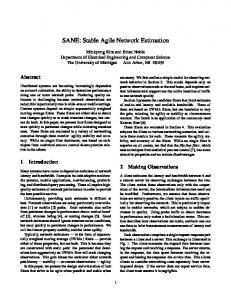
There are several cases in which empirical findings clash with what we would expect provided the theoretical assumptions made. In the specific case, we may observe that in several cases the estimation residuals turn out to have much thicker tails than those expected according to the normal law. This means that one of the two assumption we made, i.e. that the noise is given by the contribution of a high number of factors and that those factors have finite variance, must be wrong. The removal of the former is not promising since it leads to idiosyncratic models of no general interest. In this work, we shall concentrate on the second assumption. As a first example, consider the sample of audio noise depicted in figure 1. Albeit it seems natural to assume that a noise of this kind is the result of the aggregation of a large number of components, the histogram displays tails much thicker 2

Figure 1: Histogram and pattern of the audio noise sample.

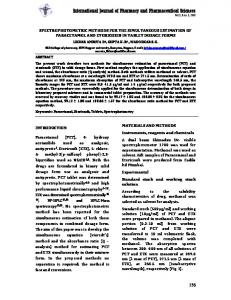
than under the Gaussian model. This could be a symptom that the variance of the components is non-finite. Let us first start by providing an useful descriptive tool for assessing the finiteness of the variance of a random vector. The variogram of a i.i.d. random sequence is defined as the vector V whose k-th entry is given by Vk =

k X ¯ k )2 (Xi − X

n−1

i=1

,

(1.2)

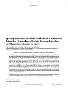
where X¯k denotes the sample mean of the first k observations; Vk is thus the sample variance of the first k items of the data-set. If the central limit theorem holds, the sample variance is a consistent estimator for the true population variance, so the variogram, provided that the sample size is large enough, should display a convergent pattern. When this does not happen, as there are “jumps” caused by observations lying on the tails that draw away the convergence, it is a symptom that the variance is non-finite. An example of a convergent and divergent pattern is provided in figure 2; the variogram of the audio noise is displayed in figure 3. Figure 2: Convergent and non-convergent variogram.

3

Figure 3: Variogram of the audio noise sample.

1.3

The generalized central limit theorem

So what should we do when the variances of the components are apparently nonfinite? The question will be answered in the following few pages2 , in which we will introduce a generalized version of the central limit theorem that relaxes the assumption of the finiteness of the variance and identifies a new family of limiting distributions, of which the normal is a particular – and definitely the much relevant – case. Let us first start by introducing a definition of the stability property. Definition 1.1 (Stability, Gnedenko & Kolmogorov 1954). The distribution function F (x) is said to be stable if for any positive numbers c1 and c2 and real numbers d1 and d2 there correspond constants c > 0 and d such that F (c1 x + d1 ) · F (c2 x + d2 ) = F (cx + d).

(1.3)

The interesting fact that constitutes the first building block of a generalized version of the central limit theorem is proven by the following theorem: stable distributions are the only possible limiting laws for normalized sums of the kind: Sn =

X1 + X2 + · · · + Xn − Dn . Cn

This result was first derived by L´evy (1924) and will be formalized in the following theorem. 2

The complete proof of the generalized central limit theorem is much more complex than the classical one and requires a strong mathematical background. Although it is covered in detail in advanced probability theory textbooks such as Feller (1966), we have decided to attempt for a “quick and dirty” approach that can help the reader to catch the blueprint of the proof without deepening too much in the mathematical details; the advanced reader will thus find several imprecisions and ambiguities. Proofs of the various theorems and lemmas are adapted – and simplified – from Gnedenko & Kolmogorov (1954), Feller (1966) and Samorodnitsky & Taqqu (1994).

4

Theorem 1.2 (L´evy3 ). Given a sequence {Xi } of i.i.d. random variables, the necessary and sufficient condition for F (x) to be the limit distribution of Pn Xi Sn = i=1 − Dn , (1.4) Cn is that F (x) be stable. Proof. We will only prove the necessity of the condition, for the sufficiency we refer to Gnedenko & Kolmogorov (1954) (page 163). Let us assume that Sn converges to a certain limiting distribution F (x): we will prove that F (x) is stable. According to the lemma presented in Gnedenko & Kolmogorov (1954) (page 146), if X has a proper distribution, then the scaling factor Cn must satisfy lim Cn = ∞

n→∞

lim

n→∞

Cn+1 Cn

= 1

Let us take two positive constants c1 and c2 such that c1 < c2 ; it is thus possible, for every ε and l ≥ lε , to pick an m such that 0≤

Cm c2 − < ε. Cl c1

Let us now take two real constants d1 and d2 and define Cn = Cl /c1 and Dn = [Cl Dl + Cm Dm + d1 Cl + d2 Cm ]/Cn . We thus may rewrite the sum (1.4) as:     Cl X1 + · · · + Xl Cm Xl+1 + · · · + Xl+m − Dl − δ1 + − Dm − δ2 . Cn Cl Cn Cm Since we have assumed that Sn converges to F (x), the two addends converge (Theorem 2, page 42, Gnedenko & Kolmogorov 1954), respectively, to F (c−1 1 x+ d1 ) and F (c−1 x + d ). On the other hand, since the limit distribution of the sum 2 2 is F (x) we need to have −1 F (x) = F (c−1 1 x + d1 ) · F (c2 x + d2 ),

so (1.3) is verified and F (x) is stable. The above theorem states just that, if a limit distribution for (1.4) exists, it must be stable; it provides no information about the conditions for such an existence: it could be the case that only distributions with finite variance display convergence, so that the normal distribution would be the only possible limiting distribution. The following result completes the characterization of the generalized version of the central limit theorem we are dealing with. Let us first introduce the concept of domain of attraction. 3

Adapted from Gnedenko & Kolmogorov (1954).

5

Definition 1.2 (Domain of attraction). If the normalized sums (1.4) admit, for suitably chosen constants, a limit distribution S we say that the Xi ’s are attracted by S; the domain of attraction of S is the set of all the distributions attracted by S. From the above definition and from the classical version of the central limit theorem, it clearly follows that every distribution with finite variance is attracted by the normal law. Now, the goal of the following theorem is to show that by replacing the condition of the finiteness of the variance with a milder one about the regular behavior of the tails, the normalized sums (1.4) admit a limit distribution. Such a distribution, because of the result of the previous theorem, has to be stable. R +x Theorem 1.3 (Generalized Central Limit4 ). Let u(x) = −x t2 dF (t) and let l(x) be a slowly varying function at infinity, namely such that, ∀x > 0: lim l(tx)/l(t) = 1.

t→∞

The distribution function F (x) belongs to the domain of attraction of a stable distribution with characteristic exponent 0 < α ≤ 2 if and only if: 1. lim u(x) = x2−α l(x); x→∞

1 − F (x) F (−x) = p and lim = q. x→∞ 1 − F (x) + F (−x) x→∞ 1 − F (x) + F (−x)

2. lim

A few remarks about the above assumptions will help to focus the situation. First, note that u(x) is a “windowed” version of the non-central second moment. The first assumption states that it may well go to infinity, but with some sort of “regular” fashion, i.e. as the product of a power term and a generic slowly varying function. In much less formal terms, nothing too strange has to happen on the road to infinity. It is possible to prove that assumption 1 is equivalent to: x2 [1 − F (x) + F (−x)] 2−α = < ∞; x→∞ u(x) α lim

(1.5)

this basically means the theorem works with thick but to some extent “regular” tails. Assumptions 2 and 3 are similar to assumption 1, but deal with the individual behavior of each tail. When X is symmetric, it follows immediately that p = q = 1 2. Proof. We will only prove the sufficiency of the above conditions, for the necessity we refer to Feller (1966) (page 304). It will be used the theorem (page 301, Feller 1966) concerning the convergence of the normalized sums (1.4). The three conditions required for the theorem to hold are5 , in this setting: 4 5

Adapted and simplified from Feller (1966). With the notation g(x) = o[f (x)] we mean that lim g(x)/f (x) = 0. x→∞

6

2

Z

+x

a. v (x) =

2 tdF (t) = o [u(x)];

−x

b. lim nt2 dFn (t) = Ω{dt}, where Ω is a generic measure; n→∞

c. n [1 − F (η) + F (−η)] < ε for all n ∈ N with η sufficiently large. Let us start by condition a. If the first moment lim v(x) does exists and the x→∞

second moment lim u(x) does not the condition is immediately verified. If both x→∞ moments exist, it is sufficient to find an appropriate constant to center the first to zero so that lim v(x) = 0. If neither moment exists, condition 1 holds if x→∞

u(x) goes to infinity faster than v 2 (x). By Schwarz’s inequality, [v(x) − v(a)]2 ≤ u(x) [1 − F (a) + F (−a)] for x > a, so the condition is verified whenever lim u(x) = ∞. x→∞ Condition c is easily seen to be a direct consequence of the alternative version (1.5) of the first assumption. It remains to check condition b. By assumption 1, it is possible to choose Cn such that: n u(Cn ) = 1 ⇒ 2 n→∞ Cn n lim 2 u(Cn x) = x2−α . n→∞ Cn lim

If α = 2, condition b is fulfilled by taking Ω concentrated at the origin. If, on the other hand, α < 2, conditions 2 and 3 assure that6 : n + u (Cn x) = px2−α , Cn2 n lim 2 u− (Cn x) = qx2−α , n→∞ Cn lim

n→∞

and the above argument extends separately to u+ (x) and u− (x). We have thus proven that the normalized sums converge to a limit. By theorem 1.2, the limiting distribution must be stable. This completes the proof. Remark 1.1. When the above limit is 0, we obtain α = 2. As we will see in what follows, this number identifies a Gaussian distribution, and the condition x2 [1 − F (x) + F (−x)] = 0, x→∞ u(x) lim

might be thought of as a relaxation of the finite variance assumption for the traditional central limit theorem. 6

We have used the shorthand notation u+ (x) =

7

R +x 0

t2 dF (t) and u− (x) =

R0 −x

t2 dF (t).

Example 1.1. As an illustration, we will now consider a distribution which is not subject to the central limit theorem in its classical version but fulfills the conditions for belonging to the domain of attraction of a stable law. The Cauchy distribution is defined as f (x) =

1 π(1 + x2 )

F (x) =

1 1 − arctan(x), 2 π

for x ∈ R; it is straightforward to show that this distribution has no mean (and therefore no higher-order moments). Let us now note that the distribution is symmetric, so that F (−x) = 1 − F (x) and apply (1.5) to obtain:   2x2 12 − π1 arctan(x) 2x2 [1 − F (x)] lim = lim 1 R +x x→∞ 1 +x t2 dt x→∞ 2 π [t − arctan(t)]−x π −x 1+t   2 2 π πx 2 − arctan(x) = lim 2 x→∞ [x − arctan(x)] ππ  x 2 − arctan(x) = lim x→∞ 1 − arctan(x) x = 1 since both the numerator and the denominator tend to one. It thus follows that sums of Cauchy random variables are attracted by a stable distribution with characteristic exponent 1 (which is itself a Cauchy distribution). As a corollary to theorem 1.3, Gnedenko & Kolmogorov (1954) report the following result about the necessary characterization of the normalizing constants Cn and Dn of (1.4). The proof, albeit simple, is quite technical and not very illustrative, so it is omitted. Corollary 1.1 (Normalizing constants). The scaling factors Cn and Dn of (1.4) must take the form √ Cn = α n (1.6)  n R +∞  √ xdF (x) if 1 < α ≤ 2   α hn −∞  1 i Dn = = ln φ n− α if α = 1    0 if α < 1 The speed of convergence issue was first addressed by DuMouchel (1973b) on the basis of an earlier theorem by Cram´er (1963). The theorem states that, given a sequence of random variables whose sum Sn converges to a stable distribution function FS (x; α), the distribution function of the sum FSn (x) is:   X FSn (x) = FS (x; α) + gk (x)n−k/α + O n−λ/α , k

8

where gk (x) is an analytic function of bounded variation which tends to 0 as x → ±∞ and the summation7 in 0 < k < min(1, ε + η) = λ includes all the numbers k = k1 α + k2 ε + k3 (2 − α) + k4 . It turns out that the term whose factor is n−k3 (2−α)/α tends to decrease very slowly when α approaches 2; the convergence to the limiting distribution can be quite very slow.

2

Stable distributions

The results of the previous section have pointed out the importance of stable distributions: although the domain of attraction of the normal law is very wide and includes all the distributions with finite variance, when we deal with phenomena with infinite variance there may well exist a limiting distribution, provided the assumptions of theorem 1.3 are fulfilled, and this limiting distribution belongs to the stable family. We will now proceed in describing the main properties and the characteristics of stable distributions.

2.1

Definitions

Although the stability property has already been defined in (1.3) we will now provide a few equivalent but much more illustrative definitions, following the approach of Samorodnitsky & Taqqu (1994). Let us start by defining a property that encompasses the stability. Definition 2.1 (Infinite divisibility). A random variable X is said to be infinitely divisible if and only if, for any n ∈ N, it can be represented as the sum of n i.i.d. random variables, namely X = Xn,1 + Xn,2 + · · · + Xn,n .

(2.1)

It clearly follows from the above definition that a sufficient condition for the infinite divisibility is that the characteristic function of X is the n-th power of some other characteristic function depending on n. For instance, it may be proven immediately that the normal, the Poisson and the Cauchy distributions are all infinitely divisible. Example 2.1. The normal distribution is infinitely divisible. If we consider a random variable X ∼ N (µ, σ 2 ) we may write it as the sum of two i.i.d. random variables X1 and X2 with N (µ/2, σ 2 /2) distribution. In general, for any given n, X may be written as the sum of n i.i.d. random variables Xi with distribution N (µ/n, σ 2 /n). 7

The symbols ε and η denote “small” quantities involved in the tail behavior of the components of the sum; for a more detailed treatment, refer to DuMouchel (1973a).

9

It may be proven (page 76, Gnedenko & Kolmogorov 1954) that the characteristic function of an infinitely divisible law is necessarily of the form:    Z +∞  itu 1 + u2 itu e −1− φ(t) = exp iδt + dG(u) , (2.2) 1 + u2 u2 −∞ where δ is a real constant and G(u) is a nondecreasing function of bounded variation. For u = 0, the integrand is defined as −t2 /2. An equivalent definition, sometimes referred to as L´evy’s formula is the following. If we define: Z u 1 + v2 M (u) = dG(v) ∀u < 0; v2 −∞ Z +∞ 1 + v2 dG(v) ∀u > 0; N (u) = v2 u σ 2 = G(0+ ) − G(0− ); we can restate (2.2) as: n φ(t) = exp iδt −

σ2 2 2 t

Z

0

+ +

h

eiut − 1 −

−∞ Z +∞ h 0

iut 1+u2

i

dM (u) +  i iut iut e − 1 − 1+u2 dN (u)

(2.3)

Let us now move, as mentioned in the introduction, to more intuitive definitions of the stable distributions. Definition 2.2 (Stability, Samorodnitsky & Taqqu 1994). A random variable X is said to have a stable distribution if and only if for any positive numbers c1 and c2 there exist a positive number c and a real number d such that cX + d = c1 X1 + c2 X2

(2.4)

where the X1 and X2 are independent and have the same distribution as X. If d = 0, X is said to be strictly stable. Please note also that the above definition is clearly equivalent to (1.3) used in the previous section. Another equivalent and even more intuitive definition which can be easily derived from (2.4) is the following: Definition 2.3 (Stability). A random variable X is said to have stable distribution if and only if for any natural number n ≥ 2 there exist a positive number Cn and a real number Dn such that X=

X1 + X2 + · · · + Xn − Dn , Cn

(2.5)

where the Xi ’s are independent copies of X. If Dn = 0, X is said to be strictly stable. 10

Essentially, this means that a random variable is stable if it can be broken up in a series of pieces identical to itself up to some normalizing constants. Given definition (2.5), it is clear that stable distributions represent a particular case of infinitely divisible distributions: contrary to what happens in (2.1), the addends are required to have all the same distribution as X scaled by the factor Cn . Example 2.2. The normal distribution is stable. Let us consider again a random variable X ∼ N (µ, σ 2 ). The sum of n independent copies of X has N (nµ, nσ 2 ) √ distribution, so if we set Cn = n and Dn = (n − 1)µ we obtain X = [X1 + X2 + · · · + Xn ]/Cn − Dn . It is worthwhile to note that, in (2.5), the equality sign holds ∀n ∈ N and not only in the limit, as it happens in the generalized central limit theorem. An alternative definition of stable distributions relying on the generalized central limit theorem and on domains of attractions is the following. Definition 2.4 (Stability, domain of attraction). A random variable X is said to be stable if it has a domain of attraction, that is if there is a sequence of i.i.d. random variables Yi such that Pn d i=1 Yi − Dn −→ X Cn for suitably chosen Cn > 0 and Dn .

2.2

Characteristic function

The most simple way to characterize stable distributions is by means of their characteristic function, whose expression will be derived in the following theorem. It is the case to note that, since the theorem works in both directions, this provides also an alternative way of defining stable distributions. Theorem 2.1 (L´evy–Khintchine). The characteristic function of a stable random variable8 S1 (α, β, γ, δ1 ) is of the form     πα if α 6= 1 exp iδ1 t − γ α |t|α 1 − iβsgn(t) tan  2 φ1 (t) = (2.6) exp iδ1 t − γ|t| 1 + iβ π2 sgn(t) ln |t| if α = 1 where 0 < α ≤ 2, −1 ≤ β ≤ 1, γ > 0 and δ ∈ R. Conversely, if a random variable has characteristic function of the form (2.6), it is stable. Proof. Let us note first that the definition of stability (1.3) may be translated, in terms of characteristic functions, as    
ln φ ct = ln φ ct1 + ln φ ct2 + iβt. 8

Subscripts will be used in order to avoid confusion with different parameterizations that will be presented later.

11

where β = (d − d1 − d2 ). Since stable distributions are infinitely divisible, we may exploit the expression (2.3) for the characteristic function and rewrite the above expression as Z 0 h i
t σ2 2 iut ln φ c = idc t − 2c2 t + eiut − 1 − 1+u 2 dM (cu) + −∞

Z

+∞ h

Z

+∞ h

i iut eiut − 1 − 1+u 2 dN (cu) ⇒ 0 Z 0 h i
σ2 2 t iut ln φ c = idc1 t − 2c2 t + eiut − 1 − 1+u 2 dM (c1 u) + +

1

+

−∞

eiut − 1 −

0

Z + +

0

h

eiut − 1 −

−∞ Z +∞ h 0

iut 1+u2

iut 1+u2

eiut − 1 −

i

i

iut 1+u2

dN (c1 u) + idc2 t −

+

dM (c2 u) +

i

dN (c2 u).

Because of the uniqueness of the representation, we conclude that: h i = 0, σ 2 c12 + c12 + c12 1

σ2 2 t 2c22

(2.7)

2

M (cu) = M (c1 u) + M (c2 u)

∀u < 0,

(2.8)

N (cu) = N (c1 u) + N (c2 u)

∀u > 0.

(2.9)

From the latter condition, we may observe that, by repeatedly exploiting the stability property, N (cu) = N (c1 u) + N (c2 u) + . . . + N (cn u) for any natural n. In particular, if we set c1 = c2 = · · · = cn = 1: N (cu) = nN (u), where c depends on n: c = c(n). A limiting argument (page 166, Gnedenko & Kolmogorov 1954) shows that the function N satisfies λN (u) = N [γ(λ)u]

∀λ > 0,

(2.10)

where the function γ(λ) is decreasing and continuous. It then follows that, excluding the case in which it is identically equal to zero, the function N (u) is different from zero everywhere. Since it may be shown that N (u) has continuous derivatives for every u, it follows from (2.10) that, if we denote N 0 (u) the first derivative of N (u), λN 0 (u) = cN 0 (cu) ⇒ N 0 (u) N 0 (cu) = c . N (u) N (cu) 12

(2.11)

0

(1) If we put u = 1 in (2.11) and we define α = − NN (1) , we obtain:

−α = c

N 0 (c) , N (c)

hence N (c) = −k2 cα ,

(2.12)

where k2 is a positive constant. Now, from the results concerning infinitely divisible distributions, we know that N (u) must fulfill two requirements: 1.

lim N (u) = 0;

u→+∞

Z 2.

∞

u2 dN (u) < +∞.

0

Since γ(λ) is decreasing, the first requirement is satisfied, according to (2.12), when α > 0. The second requirement can be written, using (2.12), as: Z ∞ k2 d u1−α du; 0

this integral converges for α < 2, so we conclude that 0 < α < 2. A similar line of reasoning leads, from (2.8), to the result: M (c) = −

k1 . |c|α

We can thus write the logarithm of the characteristic function (2.3) as: Z 0 h i 1 σ2 2 iut ln φ(t) = iδt − 2 t + k1 eiut − 1 − 1+u du 2 |u|1+α −∞ Z +∞ h i 1 iut + k2 eiut − 1 − 1+u du. 2 u1+α 0

(2.13)

(2.14)

Equations (2.11) and (2.12) together with (2.8) and (2.9) yield c−α = 2; on the other hand, when c1 = c2 = 1, we find that   2 1 − 2 = 0. σ c2 We have already pointed out that α < 2, so in order for the above equation to hold, we need that σ = 0. Equation (2.14) thus becomes: Z 0 h i 1 iut ln φ(t) = iδt + k1 eiut − 1 − 1+u du (2.15) 2 |u|1+α −∞ Z +∞ h i 1 iut + k2 eiut − 1 − 1+u du. 2 u1+α 0 13

Now, if conditions (2.8) and (2.9) are satisfied because N (u) ≡ 0 and M (u) ≡ 0, we must have k1 = k2 = 0 and, since σ > 0, c−2 = 2, so that α = 2. Equation (2.14) becomes then: 2 ln φ(t) = iδt − σ2 t2 ; (2.16) that is the characteristic function of a normal distribution. Now, setting k1 − k2 β= , k1 + k2 so that −1 ≤ β ≤ 1 and  R ∞ −u 1 if 0 < α < 1 du(k1 + k2 ) cos πα  − R0 e − 1 u1+α 2 ∞ −u 1 πα − 0 e − 1 + u u1+α du(k1 + k2 ) cos 2 if 1 < α < 2 γ=  (k1 + k2 ) π2 if α = 1

(2.17)

(2.6) follows after some tedious algebra. Remark 2.1. Note that, when α = 1, the characteristic function (2.6) contains the term ln |t|. This is a source of problems that will force us, in the following, to treat the case α = 1 separately.

2.3

Alternative parameterizations

While the characteristic function (2.6) has a quite manageable expression and can straightforwardly produce several interesting analytic results in addition to those presented in the previous subsection, unfortunately it has a major drawback for what concerns estimation and inferential purposes: it is not continuous with respect to the parameters, having a pole at α = 1. An alternative way to write the characteristic function that overcomes this problem, due to Zolotarev (1986), is the following:  
  1−α − 1 exp iδ0 t − γ α |t|α 1 + iβ tan πα if α 6= 1 2 sgn(t) |γt| φ0 (t) = if α = 1 exp iδ0 t − γ|t| 1 + iβ π2 sgn(t) ln(γ|t|) (2.18) In this case, the distribution will be denoted as S0 (α, β, γ, δ0 ). The formulation of the characteristic function is quite more cumbersome, and the analytic properties, as we will show in the following paragraphs, have less intuitive meaning. Anyway, this formulation is much more useful for what concerns statistical purposes and, unless otherwise stated, we will refer to it in what follows. The correspondence between δ1 in S1 and δ0 in S0 is given by:  if α 6= 1 δ1 + βγ tan πα 2 δ0 = (2.19) 2 if α = 1 δ1 + β π γ ln γ On the basis of the above relationship, a S1 (α, β, 1, 0) distribution corresponds to a S0 (α, β, 1, −βγ tan πα 2 ), provided that α 6= 1. 14

Another parameterization which is sometimes used is the following (Zolotarev 1986), which will be denoted as S2 (α, β2 , γ2 , δ1 ): n h io ( exp iδ1 t − γ2α |t|α exp −i πβ2 2 sgn(t) min(α, 2 − α) if α 6= 1 φ2 (t) =    2 exp iδ1 t − γ2 |t| 1 + iβ2 π sgn(t) ln(γ2 |t|) if α = 1 (2.20) Also in this case, however, the density is not continuous with respect to α and presents a pole at α = 1. Another unpleasant feature of this way of writing the characteristic function is that the meaning of the asymmetry parameter β changes according to the value of α: when α ∈ (0, 1) a negative β indicates negative skewness, whereas for α ∈ (1, 2) it produces positive skewness. For what concerns the “translation” of this parameterization into the others, we have, for α 6= 1:   πβ2 β = cot πα tan min(α, 2 − α) (2.21) 2 2 h  i1/α γ = γ2 cos πβ2 2 min(α, 2 − α) , while δ and α remain unchanged.

2.4

Meaning of the parameters

According to the results presented in the previous subsections, we have defined, for the stable family of distribution, three different analytic representation depending on four parameters: α ∈]0, 2], β ∈ [−1, 1], γ ∈ R+ and δ ∈ R; we will thus use the shorthand notation Sk (α, β, γ, δ), where k denotes the parameterization choice (0, 1 or 2). We will now describe the properties of stable distributions by the analysis of the exact meaning of each coefficient. Please recall that the difference between parameterizations 0 and 1 lies in the parameter δ, so the properties that deal with the other parameters hold for both cases. We will start by assessing that the parameter β has to do with the symmetry properties of the distribution. Property 2.1 (Reflection). Let X1 ∼ Sk (α, β, 1, 0) and X2 ∼ Sk (α, −β, 1, 0): it then follows that X2 = −X1 , therefore f2 (x) = −f1 (x) and F2 (x) = 1 − F1 (x). It thus follows that, when β = 0, the distribution is symmetric. On the other hand, when β > 0 the distributions turns out to be rightward skewed while when β < 0 it has left skewness. The cases β = ±1 correspond to a perfect positive or negative skewness: the distribution has density zero on the negative semi-axis and takes positive values on the positive semi-axis. By the following result, we will identify α as the tail-thickness parameter: as it decreases, tails tend to get thicker.

15

Property 2.2 (Tail behavior). Let X ∼ S0 (α, β, γ, δ) and α < 2. Then: Γ(α) −α sin πα , 2 (1 + β)x π Γ(α) −(α+1) lim f (x; α, β) = −αγ α sin πα . 2 (1 + β)x x→∞ π lim P(X > x) = γ α

x→∞

(2.22) (2.23)

Similar results for the left tail behavior follow straightforwardly from the reflection property. From the above result we may observe that: 1. according to (2.22), as α increases the tails get thinner; 2. in the limit, the tails behave as a power law; 3. the density of the right tail is greater than the one on the left tail as β > 0, which is consistent with our discussion of symmetry properties. Let us now move to the parameters γ and δ: we will show that they represent, respectively, scale and location of the distribution. Property 2.3 (Standardization). Let Z ∼ S1 (α, β, 1, 0); then  γZ + δ if α 6= 1
X= γZ + δ + β π2 γ ln γ + δ if α = 1 has S1 (α, β, γ, δ) distribution. If, on the other hand, Z ∼ S0 (α, β, 1, 0); then
 γ Z − β πα 2 + δ if α 6= 1 X= γZ + δ if α = 1

(2.24)

(2.25)

has S0 (α, β, γ, δ) distribution. Z is thus some sort of a standardized version of X; in the sequel, we will denote a standardized stable distribution with the shorthand notation Sk (α, β) instead of Sk (α, β, 1, 0).

2.5

Moments and moment properties

We have shown how the four parameters of stable distributions are closely related to location, scale, asymmetry and kurtosis: one may argue that there is some kind of close relationship between them and the theoretical moments. Unfortunately, it may be easily shown, by exploiting the tail behavior, that moments of order greater than α do not exist when α < 2. Property 2.4 (Moments). Let X ∼ Sk (α, β, γ, δ). Then E (|x|r ) < ∞ if and only if 0 < r < α. 16

R∞ Proof. Let us consider the quantity η xr f (x)dx, where η is an arbitrarily big positive number. Using (2.23), we may approximate it as Z ∞ xr−α−1 dx, k(α, β, γ, δ) η

where k is a finite constant depending on the parameters of the distribution. This integral clearly converges if and only if r < α. It then follows that, except for the case of the Gaussian distribution, the variance and the higher moments never exist, while the mean does when α > 1. There is, in fact, a close relationship between the mean and the location parameter, as the following property shows. Property 2.5 (Mean). Let X ∼ S1 (α, β, γ, δ) with α > 1. Then E(X) = δ.

(2.26)

If, on the other hand, X ∼ S0 (α, β, γ, δ) with α > 1. Then E(X) = δ − βγ tan πα 2 .

(2.27)

We thus observe that the location parameter coincides with the mean in parameterization 1.

2.6

Linear transformations and combinations

Let us now introduce two useful results about linear transformations and combinations of stable random variables. Property 2.6 (Linear transformations). Let X ∼ S0 (α, β, γ, δ) and a 6= 0, b ∈ R; then aX + b ∼ S0 (α, βsgn(a), |a|γ, aδ + b). (2.28) If instead X ∼ S1 (α, β, γ, δ), then  S1 (α, βsgn(a), |a|γ, aδ + b) if α 6= 1 aX + b ∼ 2 S1 (1, βsgn(a), |a|γ, aδ + b − βγ π a ln a) if α = 1

(2.29)

Property 2.7 (Linear combinations). Let X† ∼ S0 (α, β† , γ† , δ† ) and X‡ ∼ S0 (α, β‡ , γ‡ , δ‡ ) and let X† ⊥ X‡ . Then X† + X‡ ∼ S0 (α, β, γ, δ) with β =

β† γ†α + β‡ γ‡α

γ†α + γ‡α q γ = α γ†α + γ‡α  δ† + δ‡ + tan πα if α 6= 1 2 (βγ + β† γ† + β‡ γ‡ ) δ = δ1 + δ2 + π2 (βγ ln γ + β† γ† ln γ† + β‡ γ‡ ln γ2 ) if α = 1 17

(2.30)

if instead X† ∼ S1 (α, β† , γ† , δ† ) and X‡ ∼ S1 (α, β‡ , γ‡ , δ‡ ), then X† + X‡ ∼ S1 (α, β, γ, δ) with: β = γ =

β† γ†α + β‡ γ‡α γ†α + γ‡α q α γα + γα † ‡

(2.31)

δ = δ† + δ‡ . Note that γ =

q α

γ†α + γ‡α is a generalized version of the additive rule for the

variance of sums of independent random variables: σ 2 = σ†2 + σ‡2 .

2.7

Probability density and cumulative distribution functions

We claimed that stable density functions admit a closed form only in a very few special cases. In what follows, we will show, by means of the characteristic function, that the Gaussian, the Cauchy and the L´evy distributions are indeed particular cases of stable distributions whose density assumes a closed and manageable form. 2.7.1

Particular cases

Remark 2.2 (Gaussian distribution). When α = 2, the stable distribution coincides with a normal with mean δ and variance 2γ 2 . The asymmetry parameter β does not appear in the definitions. Proof. Since tan π = 0, when α = 2 the characteristic function (2.6) reduces to:  φ(t) = exp iδt − γ 2 t2 , this corresponds to the characteristic function of a normal distribution with mean δ and variance 2γ 2 . Remark 2.3 (Cauchy distribution). When α = 1 and β = 0, the stable distribution coincides with a Cauchy distribution with position δ and scale γ. Proof. Let us first recall that the probability density function of a Cauchy distribution with position parameter δ and scale parameter γ is f (x; δ, γ) =

1 n o πγ 1 + [(x − δ)/γ]2

so that the characteristic function may be written as φ(t) = eiδt−γ|t| . Now, putting α = 1 and β = 0 in (2.6), the second addend within the brackets vanishes and we obtain exactly the same result. Remark 2.4 (L´evy distribution). When α = 1/2 and β = ±1, the stable distribution coincides with a L´evy distribution with position δ and scale γ. 18

Proof. Putting α = 1/2 and β = 1 in (2.6) yields: n o p φ(t) = exp iδt − γ|t| [1 − isgn(t)] ; this corresponds to the L´evy distribution with density s γ γ/2π − 2(x−δ) f (x; δ, γ) = , 3e (x − δ)

∀ x > δ.

The case β = −1 is similar. 2.7.2

Analytic properties

Unfortunately, there are no more known cases in which the probability density function takes a closed form. Anyway, even if the density is not available, a few very important analytic properties concerning the probability density function have been derived. Property 2.8 (Continuity). Each stable distribution has continuous and infinitely differentiable probability density function. Property 2.9 (Support). The support of stable distributions is the real line when |β| = 6 1 or α ≥ 1; otherwise, the support depends on the parameterization choice. In case 1 of (2.6) it is given by [δ, +∞[ (2.32) when β = 1 and α < 1 and by ]−∞, δ] when β = −1 and α < 1; in case 0 of (2.18) it is   δ − γ tan πα 2 , +∞

(2.33)

(2.34)

when β = 1 and α < 1 and by   −∞, δ + γ tan πα 2

(2.35)

Property 2.10 (Mode). Stable distributions are unimodal. For symmetric stable distributions with 1 < α ≤ 2, the mode coincides with the mean (2.26) or (2.27); in the other cases it takes no closed form and needs to be numerically approximated9 . 9

In fact, when one comes up with a numerically approximable expression for the density function, the mode can be straightforwardly evaluated as the point at which that density function has a maximum. A more complete discussion of this topic can be found in Fofack & Nolan (1999).

19

2.7.3

Series expansion

The problem of the non-existence of a closed form for the density function has represented a major hinderance to the widespread use of stable distributions. Luckily enough, with the availability of more and more powerful computing machines, this issue may be overcome by means of approximate numerical methods. The first idea one could exploit is to invert the characteristic function in order to obtain the density.

f (x; α, β) = =

Z +∞ 1 e−itx φ(t; α, β)dt 2π −∞ Z ∞  1 −itx < e φ(t; α, β)dt . π 0

(2.36)

In principle, the above expression can be evaluated rapidly by means of a fast Fourier transform (Mittnik, Doganoglu & Chenyao 1999), but this produces only a set of abscissas with the associated densities. The smooth behavior of the actual density function needs thus to be reproduced by means of an interpolating function. In the following, we present two alternative approaches for the computation of the density function. The asymptotic behavior, as x → +∞ of the density can be devised from the asymptotic expansions of Bergstrøm (1952): f2 (x; α, β) = f2 (x; α, β) =

  +∞ 1 X Γ(kα + 1) kπα sin K(α) (−1)k−1 x−kα−1 π Γ(k + 1) 2 k=1   +∞ 1 X Γ(k/α + 1) kπα sin K(α) (−x)k−1 , (2.37) π Γ(k + 1) 2α k=1

with K(α) = α + β min(α, 2 − α); the former is an asymptotic expansion as x → +∞ for α ∈ (1, 2) and an absolutely convergent series ∀x > 0 for α ∈ (0, 1), the latter is an asymptotic expansion as x → 0+ for α ∈ (0, 1) and an absolutely convergent series ∀x > 0 for α ∈ (1, 2). Note that the above expressions do not deal with negative values of x. In this case, however, the density can be computed by simply exploiting the property f (x; α, β) = f (−x; α, −β). Note, also, that those expressions do not apply when α = 1. In this case, we have instead, for β > 0. f2 (x; α, β) =

+∞ 1X (−1)k−1 bk kxk−1 , π k=1

20

where

1 bk = Γ(k + 1)

Z 0

∞

h πi e−βu ln u uk−1 sin (1 + β)u du. 2

A quick alternative for symmetric stable distribution is also presented in McCulloch (1998b), where a fifth-order spline approximation of (2.36) with a set of pre-computed spline coefficients is employed. The following theorem10 expands (2.36) into a more manageable and easily computable expression. Let us first provide a few definitions.  −β tan πα if α 6= 1 2 ζ(α, β) = 0 if α = 1
 1 arctan β tan πα if α 6= 1 α 2 u0 (α, β) = π if α = 1
 21 π  π 2 − u0 if α < 1 0 if α = 1 c1 (α, β) =  1 if α > 1  h i α 1 α−1 cos[αu0 +(α−1)u] cos u   (cos αu0 ) α−1 sin α(u+u if α 6= 1 cos u ) 0 π  n o V (u; α, β) =   +βu   π2 2cos u exp β1 π2 + βu tan u if α = 1, β 6= 0 Theorem 2.2 (Probability density function). Let X have characteristic function (2.18); the probability density function f (x; α, β) is given by: 1

α(x−ζ) α−1 π|α−1|

πx 1 − 2β 2|β| e

Z

Z

+ π2

π 2

V (u; α, β)e−(x−ζ)

α α−1 V

(u;α,β)

du

if α 6= 1, x > ζ

−u0


Γ 1 + α1 cos u0 √ π 2α 1 + x2

if α 6= 1, x = ζ

f (−x; α, −β)

if α 6= 1, x > ζ

o n − πx V (u; 1, β) exp −e 2β V (u; 1, β) du if α = 1, β 6= 0

− π2

1 π (1 + x2 )

if α = 1, β = 0 (2.38)

Let us now move to the cumulative distribution function, whose expression will be derived in the following theorem. 10

The proof is very technical and will be omitted (cf. Nolan 1997).

21

Theorem 2.3 (Cumulative distribution function). Let X have characteristic function (2.18); the cumulative distribution function F (x; α, β) is given by: Z π α sgn(1 − α) 2 α−1 V (u;α,β) c1 (α, β) + V (u; α, β)e−(x−ζ) du if α 6= 1, x > ζ π −u0

1 π

Z

+ π2

1 u0 − 2 π

if α 6= 1, x = ζ

1 − F (−x; α, −β)

if α 6= 1, x < ζ

n o − πx exp −e 2β V (u; 1, β) du

if α = 1, β > 0

− π2 1 2

+

1 π

arctan x

if α = 1, β = 0

1 − F (x; α, −β)

if α = 1, β < 0 (2.39)

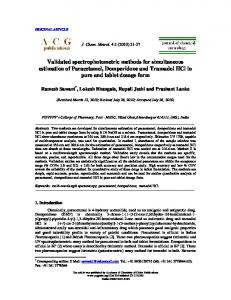
In figure 4, we report the plots of the probability density function and the cumulative distribution function for S0 (α, β) random variables for various choices of β (0,0.5,1) and α (0.5,1,1.5,1.75). 2.7.4

Numerical Problems

Let us now move to some considerations about the computational difficulties associated with the numerical evaluation of (2.38) and (2.39). The main difficulty with the evaluation of the p.d.f. and c.d.f. lies in the numerical approximation of the integral Z π α 2 α−1 V (u;α,β) V (u; α, β)e−(x−ζ) du −u0

in (2.38). Nolan (1997) points out that a more easily computable version of the density (2.38) in the case x > ζ is provided11 by: Z π 2 g(u; x, α, β)e−g(u;x,α,β) du, (2.40) f (x; α, β) = c2 (x; α, β) −u0

where

( c2 (x; α, β) =

and

( g(u; x, α, β) =

α π|α−1|(x−ζ) 1 2|β|

if α 6= 1 if α = 1

α

(x − ζ) α−1 V (u; α, β) if α 6= 1 − πx e 2β V (u; 1, β) if α = 1

11

When x = ζ the density is available in closed form and when x < ζ it follows straightforwardly from the case x > ζ according to (2.38).

22

Figure 4: Probability density function and cumulative distribution function of a S0 (α, β) random variable for different values of the parameters α and β.

23

Apart from the case when α approaches 0, in which the integration problem clearly follows from the spikedness of the probability density function, there are problems also when α is near to 1: in this case, the function V (u; α, β) varies very rapidly and so it is difficult to approximate it numerically.

2.8

Simulation

Despite the computational burden associated with the evaluation of the probability density function, stable random numbers can be straightforwardly simulated using the algorithm proposed by Chambers, Mallows & Stuck (1976). Let W be a random variable with exponential distribution of mean 1 and U an uniformly dis 
tributed random variable on − π2 , π2 . Furthermore, let ζ = arctan β tan πα 2 /α . Then    1−α  sin α(ζ + U ) cos (αζ + αU − U ) α    √ if α 6= 1   α cos αζ cos U W Z= (2.41)    π   W cos U  π  2  + βU tan U − β ln 2π if α = 1  π 2 2 + βU has S0 (α, β) distribution. Random numbers for the general case containing also the position and scale parameters δ and γ may be straightforwardly obtained using the standardization property 2.3. Similarly, random numbers with S1 (α, β, γ, δ) distribution can be readily obtained exploiting (2.19). The histogram and the summary statistics of two different simulated random vectors are reported in figure 5.

3 3.1

Stable statistical models Linear models with stable disturbances

The use of heavy tailed distributions is quite widespread in modelling the error term of linear regression models. The OLS estimation method when the distribution of the error is heavy tailed yields inefficient estimates, giving too much influence to outlying observations. To put it in more formal terms, given a n × k matrix of explanatory variables X and a k × 1 vector of parameters θ, the OLS estimator of a linear regression model in which the error term is  ∼ S1 (α, β, γ, 0) is θˆ = θ + X0 X


−1

X0 ,

and thus has infinite variance and zero efficiency with respect to a ML estimator whenever α < 2. When α > 1, however, the estimator is unbiased and consistent in probability, but the rate of convergence is n1/α−1 instead of n−1/2 .

24

Figure 5: Pattern, histogram and summary statistics for two random vectors: the first has S0 (1.8, 0.5) and the second S0 (1.5, 0) distribution.

The properties of maximum likelihood estimators were analyzed, for the symmetric case, by McCulloch (1998a). The author shows that the ML estimation of a regression model with stable disturbances can be interpreted as a weighted least squares in which the weights are decreasing with the value of the residuals (less weight given to extreme observations): w(ˆ i ) = −

3.2

∂ ln L(θ|ˆ i ) 1 . ∂θ ˆi

ARMA models

One of the most promising fields of applications of stable distributions is that of time series models. As one can in fact note, several empirical phenomena that are observed over time exhibit asymmetry and leptokurtosis (e.g. intensity and duration of rainfalls analyzed in environmetrics, activity time of CPUs and networks or noise in degraded audio samples in engineering, asset returns in finance). In this section we will show how the time series analysis paradigm of Box & Jenkins (1976) can be extended to the more general case in which the disturbances are stable rather than normal. Formally, a process is said to be ARMA (p, q) with stable innovations if it takes the form Yt =

p X i=1

ϕi Yt−i +

q X

ψj t−j + t ,

j=1

25

t ∼ i.i.d. Sk (α, β, γ, 0) ∀t.

(3.1)

A few examples of the pattern that processes of this kind can display is presented in Figure 6. Figure 6: Three ARMA (1, 1) processes with φ = 0.7 and ψ = 0.2 and stable innovations.

By defining a lag operator L such that Lk yt = yt−k , we can rewrite (3.1) as Φ(L)Yt = Ψ(L)t .

(3.2)

Provided that Φ(z) and Ψ(z) do not have common roots and that the roots of former are outside the unit circle, the process can be expressed as an infinite moving average: ∞ X Yt = cj t−j , (3.3) j=0

where the cj s are the coefficients of the series expansion of Ψ(z) Φ(z) . The proof of the above result is very simple and follows the steps of its analog in the Gaussian case. Similarly, when Ψ(L) has no roots inside the unit disk the process can be inverted, that is expressed as an infinite autoregression: ∞ X

c˜j Yt−j = t ,

(3.4)

j=0 Φ(z) where the c˜j s are the coefficients of the series expansion of Ψ(z) . From (3.3), it is straightforward to note that Yt , being a linear combination of α-stable random variables, is α-stable too with the same characteristic index. It is also immediate to observe that the sequence (3.3) is strictly stationary; however it is important to remark that, with an variance infinite, the concept of covariance stationarity is meaningless. As we have already remarked, the most striking difference with the Gaussian family of ARMA processes is that, since the variance does not exists, one cannot use the autocovariance function in order to describe the dependence structure of the process. This issue was addressed in Kokoszka & Taqqu (1994), who introduce a new concept that can be used as a proxy of the autocovariance function. Define the autocovariation function as: h i h i h i Ik (θ1 , θ2 ) = − ln E ei(θ1 Xt +θ2 Xt−k ) + ln E eiθ1 Xt + ln E eiθ2 Xt−k . (3.5)

26

In the Gaussian case, the above expression yields Ik (θ1 , θ2 ) = θ1 θ2 Cov(Xt , Xt−k ),

(3.6)

so the function is proportional to the autocovariance. In the infinite variance case, however, the function still retains a practical meaning. Consider two stable ARMA processes {Xt } and {Yt } with the same parameters of the underlying distribution. We will show that, if {Xt } has more autocovariation than {Yt }, namely (x)

(y)

Ik (1, −1) ≥ Ik (1, −1),

(3.7)

for every k, the process {Xt } is less self-dependent than {Yt }. Let us first set h i µk = − ln E ei(Xt −Xt−k ) , (3.8) h i νk = − ln E ei(Yt −Yt−k ) . Substituting (3.8) and (3.5) into (3.7) yields µk ≥ νk and µ−1 k νk ≤ 1. X −X

Now, since t µk t−k and for any given c > 0:

Yt −Yt−k µk

have the same distribution, we can observe that,

  Xt − Xt−k > c P (|Xt − Xt−k | > c) = P µk µk   Yt − Yt−k c = P > νk µk
= P |Yt − Yt−k | > cµ−1 k νk ≥ P (|Yt − Yt−k | > c) . The above inequality means that Yt and Yt−k are less likely to be different than Xt and Xt−k and so are more dependent. An important result (Kokoszka & Taqqu 1994) concerning the dependence structure of the process is that, if the coefficients of the MA(∞) representation satisfy |cj | < M −j , then the autocovariance function decreases exponentially and so the resulting process is short memory. A more detailed analysis concerning the memory properties of stable time series can be found in Kokoszka & Taqqu (1995) and Kokoszka & Taqqu (1996).

27

3.3

Model selection and diagnostics

When dealing with “traditional” ARMA models, it is customary practice to use the correlogram in order to gain insights about the number of lags to be used. In the stable case, and more in general in every situation in which the variance of the noise is infinite, however, the non-existence of the autocovariance makes this approach a little troublesome. Suggestions in the literature have exploit the results about Gaussian ARMA processes to construct proxies of the autocorrelation function that are computed the same way but do not necessarily retain the same meaning. As an example, take a MA(∞) Gaussian process. Being the ratio of the autocovariance and the variance, the autocorrelation function depends only on the MA parameters and is given by P+∞ j=0 ψj ψj−k ρk = P+∞ 2 . (3.9) j=0 ψj Since in our case the variance does not exists, we cannot talk about autocorrelation, but we can still compute (3.9), by simply plugging in it the actual MA parameters, and call it pseudo-autocorrelation function. One could thus compute the sample analog of (3.9) P+∞ ˆ ˆ j=0 ψj ψj−k ρˆk = P+∞ . (3.10) ˆ2 j=0 ψj and “hope” that it somehow has to do with the dependence structure of the process in order to get some insights about specification issues. Luckily enough, Davis & Resnick (1986) proved that the sample autocorrelation is consistent for the pseudoACF, but the main problem lies in the fact that the asymptotic distribution of ρˆk −ρk is: 1. unknown, 2. attained very slowly as the sample size increases. The former problem poses difficulties in the fact that the confidence bounds for the empirical autocorrelation must be determined by simulation and depend on α, which is in general unknown at the model selection stage. The latter causes the actual percentage of rejections of the null hypothesis to be fairly different from the expected. Adler, Feldman & Gallagher (1998) thus propose the use of Cauchy bounds as a conservative strategy. Their simulation study showed that both the autocorrelation and the partial autocorrelation function are useful in identifying the appropriate AR and MA orders 69% of the times when using Gaussian bounds and 83% with Cauchy bounds. Another widely used model selection criterion is the Akaike information criterion (AIC), defined as: ln T 2 ln L − +k , T T 28

where k is the number of ARMA parameters. The performance of this criterion when dealing with infinite-variance models is analyzed by Knight (1989). Surprisingly enough, even if the properties of the AIC as a model selection device are based on a Gaussian likelihood function, its performance is even improved when the tails of the actual distribution of the noise get thicker.

4

Estimation and inference

Despite their appealing theoretical properties and the obvious inadequacy of the Gaussian assumption for a wide number of applied situations, stable distributions have encountered a strong hinderance to their diffusion in applied statistics because of the lack of properly working estimation procedures, mainly caused by the absence of the density in closed form. In this section we will briefly review the estimation procedures that have been proposed in the literature.

4.1

Quantile-based methods

The first idea exploited to estimate the parameters of stable distributions, in particular the “tail-thickness” parameter α, was to resort to quantile-based procedures. The first contributions in this direction have focused on symmetric stable distributions. Fama & Roll (1968) show that the location parameter δ may be unbiasedly estimated by a truncated mean, that is the mean of the “central” portion of the sample; they propose, for practical applications, to use a 50% truncated mean when it is known that α lies between 0 and 2. In a subsequent article (Fama & Roll 1971) the authors show how to estimate γ and α. For what concerns the scale parameter, they observe that the 0.72 quantile of a S1 (α, 0) distribution is very close (±0.003) to 0.827 independently of α, so they propose γˆ =

qˆ.72 − qˆ.28 . 2 · 0.827

(4.1)

Since this estimator is a linear combination of order statistics, it has asymptotically normal distribution. A Monte Carlo study points out that its asymptotic bias is less than 0.4%. A similar procedure is applied to the estimation of α. Since this parameter determines the tail behavior of the distribution, one can use zˆf =

qˆf − qˆ1−f 2ˆ γ

(4.2)

and then search an appropriate table for a value α ˆ whose theoretical quantile matches zˆf . The choice of f is a difficult issue. Since the estimation procedure deals with the tail behavior, one must choose a sufficiently large f ; on the other hand, too high values of f tend to increase the sample dispersion. A Monte Carlo study reveals that values ranging from 0.95 to 0.97 are robust against variation of the “true” α. 29

A more refined and extended quantile-based estimation procedure was later proposed by McCulloch (1986). Let us consider a S1 (α, β, γ, δ) distribution. The quantities να = νβ =

q.95 − q.05 q.75 − q.25 q.95 + q.05 − 2q.5 q.95 − q.05

(4.3)

do not depend on γ and δ and are tabulated by the author as a function of α and β. The estimation of the two parameters is thus based on matching the sample analogs of the above expressions with their theoretical counterparts. Once we have obtained estimates for α and β, we can move to the estimation of the scale parameter γ. The quantity q.75 − q.25 νγ = γ has been tabulated as a function of α and β, so γˆ =

qˆ.75 − qˆ.25 . ˆ νγ (ˆ α, β)

(4.4)

Finally, the position parameter δ may be estimated as follows. Let us first consider the transformation  δ + βγ tan πα if α 6= 1 2 ζ= δ if α = 1. The quantity νζ =

ζ − q.5 γ

ˆ and has been tabulated as a function of α and β, so ζˆ = qˆ.5 + γˆ νζ (ˆ α, β) ˆγ tan πα . δˆ = ζˆ − βˆ 2

(4.5)

The above estimators are consistent but are not efficient. Furthermore, this kind of approach cannot be readily extended to linear and time series models and thus requires a two-step estimation procedure.

4.2

Characteristic function-based methods

The idea of estimating the stable distributions parameters by means of the empirical characteristic function dates back to Press (1972) and Paulson, Holcomb & Leitch (1975). The idea behind this approach is to numerically minimize, with respect to the parameters, an appropriate distance criterion between the empirical and

30

the theoretical characteristic function. Given a sample y of n units, the empirical characteristic function is n

n

j=1

j=1

X 1X ˆ = 1 φ(t) eityj = [cos(tyj ) − i sin(tyj )] . n n The approach consists thus in minimizing Z +∞ 2 ˆ φ(t) − φ(t) w(t)dt

(4.6)

(4.7)

−∞

with respect to the stable parameters, where w(t) is an appropriate weighing func2 tion. The authors suggest, for computational reasons, w(t) = e−t ; and the integral in (4.7) is computed by means of numerical quadrature. The simulation study carried out by the authors reports success of the estimation procedure only for values of γ and δ close, respectively, to 1 and 0. So, they propose a sort of two-step procedure in which rough estimators of the position and the scale parameters are obtained and then the estimation is carried out on the standardized sample values. A different approach was proposed by Koutrouvelis (1980). The author notes that the logarithm of the characteristic function in parameterization 1 (2.6) may be expressed, for α 6= 1, as:   ln φ1 (t) = − |γt|α + i δt + |γt|α sgn(t)β tan πα (4.8) 2 . The real part of the above expression is thus < [ln φ1 (t)] = −γ α |t|α , so that ln {−< [ln φ1 (t)]} = α ln |t| + α ln γ.

(4.9)

Similarly, the imaginary part of (4.8) can be expressed as = [ln φ1 (t)] = δt + |γt|α sgn(t)β tan πα 2 .

(4.10)

The proposed approach is therefore to: 1. Estimate γ and δ by means of a quantile method and standardize the data. 2. Compute the empirical characteristic function (4.6) and the sample analogs of (4.9) and (4.10) by means of i  h  < φˆ1 (t)  h i h i h i . < ln φˆ1 (t) = ln φˆ1 (t) = ln φˆ1 (t) = arctan  = φˆ (t)  1 The points at which the characteristic function is evaluated are determined on the basis of a lookup table (Koutrouvelis 1980). 31

n h io 3. Regress ln −< ln φˆ1 (t) on a constant and ln |t| (cf. 4.9); dividing the constant by α ˆ is the basis for an update of γˆ . 4. Regress the imaginary part of the empirical characteristic function on a constant and t (cf. 4.10) to get an estimate of β and an update for δ. This approach was later improved in Koutrouvelis (1981) by means of an iterated GLS regression with the covariances of the regression errors as weights. A more refined technique exploiting the characteristic function was recently proposed by Kogon & Williams (1998). The authors resort to the parameterization 0 of the characteristic function (2.18). The regression equations, as in the previous case, are thus: ln {−< [ln φ0 (ti )]} = α ln |ti | + α ln γˆ + ui , (4.11)   ˆ ˆ i + βˆ ˆγ ti tan πα |ˆ = [ln φ0 (ti )] = δt γ ti |α−1 − 1 + vi . 2 Besides the use of a different parametrization, the difference between this approach and that of Koutrouvelis (1980) lies in the choice of the points at which the characteristic function is evaluated. Instead of the lookup table, Kogon & Williams (1998) use a fixed interval independent on the scale and the location parameters. This interval is determined by observing that the sample characteristic function is deterministic and equal to its theoretical counterpart at t = 0, so the proposed optimal interval is t ∈ [0.1, 1.0]. A simulation exercise shows that the optimal number of equally spaced points in which the above interval should be divided is 10. A detailed simulation study points out that this estimator performs, in general, quite remarkably, and tends to outperform the quantile method (McCulloch 1986). Its performance is however worse than that of the GLS method of Koutrouvelis (1981), especially when α is small. Nevertheless, this loss of accuracy is compensated by its simpler formulation, since it does not require the use of the lookup tables nor an iterative procedure.

4.3

Maximum likelihood

The potential of the maximum likelihood approach was first advocated by DuMouchel (1973a), who showed that the estimator follows the standard asymptotic theory. However, the author notes that the likelihood function has weird behavior since lim L(x; α, δ) = +∞. α→0, x→δ

It thus displays poles whenever the observed value approaches the location parameter δ. When δ is known, this obviously does not happens, since P(X = δ) = 0. This problem can be overcome by restricting the admissible values of α to ε < α ≤ 2, with ε arbitrarily small. Since the likelihood function has a discontinuity at α = 1, we will also exclude this parameter value. We will denote the restricted sample space as Θ, and C will be an arbitrary open subset of Θ. 32

The proof of the asymptotic normality and consistency of the maximum likelihood estimator is based on the conditions of LeCam (1952): 1. The density f (x; θ) is continuous ∀θ ∈ Θ and has continuous first and second partial derivatives ∀x and ∀θ0 ∈ C c , where C c denotes the complement of C. 2. The joint density of the sample is such that: Qn   f (xi ; θ) i=1 Eθ0 sup ln Qn 0. 6. The information matrix is nonsingular ∀θ ∈ C c . The proof that the above conditions hold is given by DuMouchel (1973a), allowing to establish the following theorem. Theorem 4.1 (Maximum likelihood estimator). The maximum likelihood estimator is consistent and asymptotically normal with variance-covariance matrix I−1 (θ) as long as θ ∈ Θ. In practice, the normal approximation works only for certain values of α and β: when the two parameters are close to their bounds, the asymptotic distribution of the maximum likelihood tends to become degenerate for a fixed sample size. Nevertheless, this result is very promising and, in principle, should lead to prefer the maximum likelihood over the others approaches outlined in the previous section. Unfortunately, this approach was markedly hindered by the absence of the density in closed form, so that the evaluation of the likelihood function requires the numerical inversion of the characteristic function for every different parameter vector and thus may be very time-consuming. The first proposal to overcome this computational difficulty was put forth by DuMouchel (1971): he proposes to divide the data in intervals of fixed width and then compute the inverse fast Fourier transform to obtain the density of “central”

33

groups of observations and the asymptotic expansion (2.37) for the “extreme” observations. The loss of information associated with this grouping technique is analyzed in DuMouchel (1975). Two approaches to the practical computation of maximum likelihood estimates have been recently proposed: the first one, due to Nolan (2002), exploits the series representation of Nolan (1997) reported in (2.40); the other, first employed by Mittnik, Rachev, Doganoglu & Chenyao (1999), use a linear interpolation of the fast Fourier transform of the characteristic function (Mittnik, Doganoglu & Chenyao 1999). Both approaches report a significant reduction of the mean squared error with respect to the quantile method of McCulloch (1986).

5

Tests for stable behavior

In principle, since they have four parameters instead of two, there should be no doubt that stable distributions fit data better than the normal. In several cases, however, empirical data distributions are not too far from the Gaussian; it thus becomes crucial to devise testing methodologies able to discern between the two distributions12 . The problem of the choice between a normal and a more general stable specification was first addressed by DuMouchel (1983). As we pointed out in the previous paragraph, the maximum likelihood estimator follows the standard asymptotic theory for values within the bounds of the parameter space. On the other hand, when α approaches 2, the estimator becomes super-efficient, that is its standard error tends to zero for a fixed sample size: this is obviously a major problem in a testing framework. However, the author shows that lim P(ˆ α = 2) = 1.

n→∞

A simulation exercise, in which normal observations were fitted by a stable model, considers thus the properties of the simple test constructed by means of the rule “reject whenever α ˆ < 2”. It appears that, with a sample size of 1000 observations, the test incurs in a type I error 16% of the times. The author further conjectures that k P(ˆ α = 2) ≈ , ln n where k is a constant term, so that one should need a few millions of observations before the test attains a 5% significance level. Because of this difficulty, testing procedures have focused on visual techniques. Besides the already mentioned variogram, several authors have developed alternative testing strategies: Nolan (2002), for example, analyzes the use of q-q and p-p plots. 12 A very useful survey on testing methodologies is provided in Nardelli (1997) and has greatly inspired this section.

34

Some authors (Fama & Roll 1971) have tried to exploit the stability property: if a dataset is stable, aggregations should be stable too and exhibit the same stability index. This approach has led to the rejection of the stability assumption for several phenomena, since it is often found that, as the aggregation level moves on, α approaches 2. This testing methodologies cannot be considered appropriate for two reasons: first, as Diebold (1986) points out, what we actually reject is the fact that the random variables are not i.i.d. stable, they could well be stable with different parameters; second, as shown by Fielitz & Smith (1971), if the actual data is generated by mixtures of stable distributions with different scale and location, the estimated α will tend to grow with the aggregation level. In most cases, however, practitioners focus one the tail behavior of the distribution: it is common to stumble in plots of the empirical distribution on a log-log scale that are used to justify the employment of a stable model by noting the power (linear on a log-log scale) decay of the tails. Besides the fact of not being formal and not dealing with the “central” part of the distribution, which could well be very far from being stable, this method is prone to error and should be avoided because, as already noted in property 2.2, the power decay of the tails occurs asymptotically and is difficult to decide when x gets large enough to justify it. A widely employed test that deals with tail behavior is the so-called Hill plot (Hill 1975). The idea is to recursively compute n 1 X hk = ln x(i) − ln x(n−k) k

"

#−1 (5.1)

i=n−k

for k = 1, . . . , n and see how this quantity behaves. If the tails have power decay, this quantity should approach the exponent, and thus constitute an estimate of α for stable distributions. This approach is very simple and has encountered a large fortune. Since several empirical studies have found α ˆ > 2, this has been interpreted as evidence against the stable model. This line of reasoning was strongly criticized by McCulloch (1997), who shows that stably-distributed samples with α as small as 1.65 can well yield an α ˆ > 2. In the same paper, the critical values of the LR statistic under the null hypothesis α = 2 are tabulated, making thus possible the use of the likelihood ratio in order to discern between the normal and the stable model.

References Adler, R., Feldman, R. & Gallagher, C. (1998), Analysing stable time series, in R. Adler, R. Feldman & M. Taqqu, eds, ‘A practical guide to heavy tails’, Birkh¨auser, Berlin. Bergstrøm, H. (1952), ‘On some expansions of stable distribution functions’, Arkiv f¨ur Mathematik 2, 375–378.

35

Box, G. & Jenkins, F. (1976), Time Series Analysis: Forecasting and Control, Holden-Day, San Francisco. Chambers, J., Mallows, C. & Stuck, B. (1976), ‘A method for simulating stable random variables’, Journal of the American Statistical Association 71, 340– 344. Cram´er, H. (1963), ‘On asymptotic expansions for sums of independent random variables with a limiting stable distribution’, Sankhya 25, 13–24. Davis, R. & Resnick, S. (1986), ‘Limit theory for the sample covariance and correlation functions of moving averages’, Annals of Statistics 14, 533–558. Diebold, F. (1986), Temporal aggregation of ARCH processes and the distribution of asset returns, Special Studies Paper 200, Board of Governors of the Federal Reserve System. DuMouchel, W. (1971), Stable Distributions in Statistical Inference, PhD thesis, Yale University, New Haven. DuMouchel, W. (1973a), ‘On the asymptotic normality of the maximum-likelihood estimate when sampling from a stable distribution’, Annals of Statistics 1, 948–957. DuMouchel, W. (1973b), ‘Stable distributions in statistical inference: 1. Symmetric stable distributions compared to other symmetric long-tailed distributions’, Journal of the American Statistical Association 68, 469–477. DuMouchel, W. (1975), ‘Stable distributions in statistical inference: 2. Information from stably distributed samples’, Journal of the American Statistical Association 70, 386–393. DuMouchel, W. (1983), ‘Estimating the stable index α in order to measure tail thickness: A critique’, Annals of Statistics 11, 1019–1031. Fama, E. & Roll, R. (1968), ‘Some properties of symmetric stable distributions’, Journal of the American Statistical Association 63, 817–836. Fama, E. & Roll, R. (1971), ‘Parameter estimates for symmetric stable distributions’, Journal of the American Statistical Association 66, 331–338. Feller, W. (1966), An Introduction to Probability Theory and its Applications, John Wiley & Sons, New York. Fielitz, B. & Smith, E. (1971), ‘Asymmetric stable distributions of stock price changes’, Journal of the American Statistical Association 67, 813–814. Fofack, H. & Nolan, J. (1999), Tail behavior, modes and other characteristics of stable distributions. American University, Washington. 36

Gnedenko, B. & Kolmogorov, A. (1954), Limit Distributions for Sums of Independent Random Variables, Addison-Wesley, Reading. Hill, B. (1975), ‘A simple general approach to inference about the tail of a distribution’, Annals of Statistics 3, 1163–1174. Knight, K. (1989), ‘Consistency of Akaike’s information criterion for infinite variance autoregressive processes’, Annals of Statistics 17, 824–840. Kogon, S. & Williams, D. (1998), Characteristic function based estimation of stable distribution parameters, in R. Adler, R. Feldman & M. Taqqu, eds, ‘A practical guide to heavy tails’, Birkh¨auser, Berlin. Kokoszka, P. & Taqqu, M. (1994), ‘Infinite variance stable ARMA processes’, Journal of Time Series Analysis 15, 203–220. Kokoszka, P. & Taqqu, M. (1995), ‘Fractional ARIMA with stable innovations’, Stochastic Processes and Their Applications 60, 19–47. Kokoszka, P. & Taqqu, M. (1996), ‘Parameter estimation for infinite variance fractional ARIMA’, Annals of Statistics 24, 1880–1913. Koutrouvelis, I. (1980), ‘Regression-type estimation of the parameters of stable laws’, Journal of the American Statistical Association 75, 919–928. Koutrouvelis, I. (1981), ‘An iterative procedure for the estimation of the parameters of stable laws’, Communications in Statistics – Simulation and Computation 10, 17–28. LeCam, L. (1952), On Some Asymptotic Properties of Maximum-Likelihood Estimates and Related Bayes Estimates, PhD thesis, University of California, Berkeley. L´evy, P. (1924), ‘Th´eorie des erreurs de la loi de Gauss et les lois exceptionnelles’, Bulletin de la Soci´et´e de France 52, 49–85. McCulloch, J. (1986), ‘Simple consistent estimators of stable distribution parameters’, Communications in Statistics – Simulation and Computation 15, 1109– 1136. McCulloch, J. (1997), ‘Measuring tail thickness to estimate the stable index α: A critique’, Journal of Business & Economic Statistics 15, 74–81. McCulloch, J. (1998a), Linear regression with stable disturbances, in R. Adler, R. Feldman & M. Taqqu, eds, ‘A practical guide to heavy tails’, Birkh¨auser, Berlin. McCulloch, J. (1998b), Numerical approximation of the symmetric stable distribution and density, in R. Adler, R. Feldman & M. Taqqu, eds, ‘A practical guide to heavy tails’, Birkh¨auser, Berlin. 37

Mittnik, S., Doganoglu, T. & Chenyao, D. (1999), ‘Computing the probability density function of the stable Paretian distribution’, Mathematical and Computer Modelling 29, 235–240. Mittnik, S., Rachev, S., Doganoglu, T. & Chenyao, D. (1999), ‘Maximum likelihood estimation of stable Paretian models’, Mathematical and Computer Modelling 29, 275–293. Nardelli, S. (1997), Statistical tests for stable distributions, Master’s thesis, European University Institute, Fiesole. Nolan, J. (1997), ‘Numerical computation of stable densities and distribution functions’, Communications in Statistics – Stochastic Models 13, 759–774. Nolan, J. (2002), Maximum likelihood estimaton and diagnostics for stable distributions. American University, Washington. Paulson, A., Holcomb, E. & Leitch, R. (1975), ‘The estimation of the parameters of the stable laws’, Biometrika 62, 163–170. Press, S. (1972), ‘Estimation of univariate and multivariate stable distributions’, Journal of the American Statistical Association 67, 842–846. Samorodnitsky, G. & Taqqu, M. (1994), Stable Non-Gaussian Random Processes, Chapman & Hall, Boca Raton. Zolotarev, V. (1986), One-dimensional Stable Distributions, American Mathematical Society, Providence.

38

Indirect inference for α-stable distributions and processes∗

Abstract The α-stable family of distributions constitutes a generalization of the Gaussian distribution, allowing for asymmetry and thicker tails. Its practical usefulness is coupled with a marked theoretical appeal, given that it stems from a generalized version of the central limit theorem in which the assumption of the finiteness of the variance is replaced by a much less restrictive one concerning a somehow regular behavior of the tails. Estimation difficulties have however hindered its diffusion among practitioners. Since simulated values from α-stable distributions can be straightforwardly obtained, the indirect inference approach could prove useful to overcome these estimation difficulties. In this paper I will provide a description of how to implement such a method by using the skew-t distribution of Azzalini & Capitanio (2003) as an auxiliary model. The indirect inference approach will be introduced in the setting of the estimation of the distribution parameters and then extended to linear time series models with stable disturbances. The performance of this estimation method is then assessed on simulated data. An application on time-series models for the inflation rate concludes the paper.

1

Introduction

The central limit theorem is one of the cornerstones of statistical inference. In the formulation provided by Lindeberg and L´evy, it basically states that, given a sequence of n independent and identically distributed random variables with finite variance, their sum converges, as n grows, to a normal distribution regardless of the individual shape. This is of crucial importance in statistical inference for two basic reasons: – most of the sample statistics are built by adding up random variables referred to the individuals in the sample. ∗ A preliminary version of this paper was presented at the conference S.Co. 2003 in Treviso. Special thanks go to Giorgio Calzolari for his help at the implementation stage. I also thank Adelchi Azzalini, Silvano Bordignon and Mauro Grigoletto for their insightful comments on a preliminary version of this work.

39

– several phenomena of statistical interest may be thought as aggregations of contributions of smaller factors. The consequence of this result is that the normal distribution is quite widespread both in statistical inference and in statistical modelling. As an example, if we hypothesize that the noise term in regression and time series models is the result of a large number of small effects with finite variances, its distribution should be normal. Since it turns out that the estimation residuals are often roughly normallike, the theoretical property of the normal distribution as a limit law matches with the empirical evidence: these two aspects support and encourage the widespread use of the normal distribution in statistical applications. However, there are situations in which empirical findings clash with what one would expect provided the theoretical assumptions made. In the specific case, one may observe that in some cases the estimation residuals turn out to have much thicker tails than those expected according to the normal law. This means that one of the two assumption we made, i.e. that the noise is given by the contribution of a high number of factors and that those factors have finite variance, must be wrong.

1.1

Stable Distributions

When the central limit theorem fails because of the non-finiteness of the variance, one should not expect anymore the Gaussian distribution as a limit law. Instead, provided that the following condition concerning the tail behavior x2 [1 − F (x) + F (−x)] 2−α = < ∞, x→∞ u(x) α lim

(1.1)

where u(x) is a slowly varying function, holds, one should observe a α-stable limiting distribution. This generalized version of the central limit theorem and the related family of distributions were introduced by Gnedenko & Kolmogorov (1954); the Gaussian distribution is thus a particular case of α-stable distribution. This family of distributions has a very interesting pattern of shapes, allowing for asymmetry and thick tails, that makes them suitable for the modelling of several phenomena; moreover, it is closed under linear combinations. The family is identified by means of the characteristic function     πα exp iδ1 t − γ α |t|α 1 − iβsgn(t) tan  if α 6= 1 2 φ1 (t) = (1.2) 2 exp iδ1 t − γ|t| 1 + iβ π sgn(t) ln |t| if α = 1 which depends on four parameters: α ∈ (0, 2], measuring the tail thickness (thicker tails for smaller values of the parameter), β ∈ [−1, 1] determining the degree and sign of asymmetry, γ > 0 (scale) and δ1 ∈ R (location). While the characteristic function (1.2) has a quite manageable expression and can straightforwardly produce several interesting analytic results, it unfortunately has a major drawback for what concerns estimation and inferential purposes: it is not continuous with respect to the parameters, having a pole at α = 1. 40

An alternative way to write the characteristic function that overcomes this problem, due to Zolotarev (1986), is the following: 
   exp iδ0 t − γ α |t|α 1 + iβ tan πα sgn(t) |γt|1−α − 1 if α 6= 1 2 φ0 (t) = 2 exp iδ0 t − γ|t| 1 + iβ π sgn(t) ln(γ|t|) if α = 1 (1.3) In this case, the distribution will be denoted as S0 (α, β, γ, δ0 ). The formulation of the characteristic function is, in this case, quite more cumbersome, and the analytic properties have less intuitive meaning. Anyway, this formulation is much more useful for what concerns statistical purposes and, unless otherwise stated, I will refer to it in the following. The only parameter that takes needs to be “translated” according to the following relationship is δ:  δ1 + βγ tan πα if α 6= 1 2 δ0 = (1.4) δ1 + β π2 γ ln γ if α = 1 On the basis of the above equations, a S1 (α, β, 1, 0) distribution corresponds to a S0 (α, β, 1, −βγ tan πα 2 ), provided that α 6= 1. Unfortunately, (1.2) and (1.3) cannot be analytically inverted to yield a closedform density function except for a very few cases: α = 2, corresponding to the normal distribution1 , α = 1 and β = 0, yielding the Cauchy distribution, and α = 12 , β = ±1 for the L´evy distribution. This difficulty, coupled with the fact that moments of order greater than α do not exist whenever α 6= 2, has made impossible the use of standard estimation methods such as maximum likelihood and the method of moments. Researchers have thus proposed alternative estimation procedures, mainly based on quantiles (McCulloch 1986) or on the empirical characteristic function (Koutrouvelis 1980), the performance of which is judged unsatisfactory in a number of respects. With the availability of powerful computing machines, it has become possible to employ computationally-intensive estimation methods for the estimation of αstable distributions; in particular, likelihood-based inference has been carried out by approximating the density with the FFT of the characteristic function (Mittnik, Doganoglu & Chenyao 1999) or with numerical quadrature (Nolan 1997). However, the accuracy of both these approximations is quite poor for small values of α because of the spikedness of the density function. The latter method, furthermore, is of very difficult implementation. Despite the computational burden associated with the evaluation of the probability density function, stable random numbers can be straightforwardly simulated using the algorithm proposed by Chambers, Mallows & Stuck (1976). Let W be a random variable with exponential of mean 1 and U an uniformly dis π πdistribution 
tributed random variable on − 2 , 2 . Furthermore, let ζ = arctan β tan πα 2 /α . 1

Note, though, that in this case β becomes unidentified.

41

Then

Z=

   1−α  sin α(ζ + U ) cos (αζ + αU − U ) α    √   α cos αζ cos U W

if α 6= 1

   π   W cos U  2 π  2  + βU tan U − β ln π  π 2 2 + βU

if α = 1

(1.5)

has S0 (α, β, 1, 0) distribution. Random numbers for the general case containing also the position and scale parameters δ and γ may be straightforwardly obtained exploiting the fact that, if X ∼ S(α, β, γ, δ), then Z = X−δ ∼ S(α, β, 0, 1). γ Similarly, random numbers with S1 (α, β, γ, δ) distribution can be readily obtained using (1.4).

1.2

Stable ARMA Processes

One of the most promising fields of applications of stable distributions is that of time series models. As one can in fact note, several empirical phenomena that are observed over time exhibit asymmetry and leptokurtosis (e.g. intensity and duration of rainfalls analyzed in environmetrics, activity time of CPUs and networks or noise in degraded audio samples in engineering, asset returns in finance). Formally, a process is said to be ARMA (p, q) with stable innovations if it takes the form Yt =

p X i=1

ϕi Yt−i +

q X

ψj t−j + t ,

t ∼ Sk (α, β, γ, 0) ∀t, k = 0, 1, 2. (1.6)

j=1

By defining a lag operator L such that Lq yt = yt−q , it is possible to rewrite (1.6) as Φ(L)Yt = Ψ(L)t . (1.7) Provided that Φ(z) and Ψ(z) do not have common roots and that the roots of former are outside the unit circle, the process can be expressed as an infinite moving average: ∞ X cj t−j , (1.8) Yt = j=0

where the cj s are the coefficients of the series expansion of Ψ(z) Φ(z) . From (1.8), it is straightforward to note that Yt , being a linear combination of α-stable random variables, is α-stable too with the same characteristic index (Samorodnitsky & Taqqu 1994). It is also immediate to observe that the sequence (1.8) is strictly stationary; however it is important to remark that, being the variance infinite, the concept of covariance stationarity is meaningless. It can be also demonstrated (Kokoszka & Taqqu 1994) that the cj s decrease at an exponential rate, so that there exists a M > 1 such that |cj | < M −j and the resulting process is short memory. 42

Since the variance does not exists, however, one cannot use the autocovariance function in order to describe the dependence structure of the process and get insights about an appropriate specification as in the Gaussian case. Methods to identify the appropriate order of AR and MA lags to be used are discussed in Nardelli (1997).

2

Indirect Inference

The indirect inference (Gouri´eroux, Monfort & Renault 1993) is an inferential approach which is suitable for every situation in which the estimation of the statistical model of interest is too difficult to be performed directly. It was first motivated by econometric models with latent variables, but it can be applied in virtually every situation in which the direct maximization of the likelihood function turns out to be difficult. The principle2 on the basis of which the indirect inference works is very simple: suppose we have a sample of T observations y and a model whose likelihood function L? (y; θ) is difficult to handle and maximize; the model could also depend on a matrix of explanatory variables X. The maximum likelihood estimate of θ ∈ Θ, given by T X ln L? (θ; yt ), θˆ = max θ∈Θ

t=1

is thus unavailable. Let us now take an alternative model, depending on a parameter vector ζ ∈ Z, which will be indicated as auxiliary model, easier to handle, and suppose we decide to use it in the place of the original one. Since the model is misspecified, the estimator ζˆ = max ζ∈Z

T X

˜ yt ), ln L(ζ;

t=1

is not necessarily consistent: the idea is to exploit simulations performed under the original model to correct for the bias. The first step consists of computing the maximum likelihood estimate of ζ, ˆ Next, one simulates a set of S vectors of size T from which will be denoted as ζ. the original model on the basis of an arbitrary parameter vector θˆ(0) . Let us denote each one of those vectors as ys (θˆ(0) ). The simulated values are then estimated using the auxiliary model, yielding ζˆS (θˆ(0) ) = max ζ∈Z

2

S X T X

h i ln L˜ ζ; yts (θˆ(0) ) .

(2.1)

s=1 t=1

This section was strongly inspired by the fourth chapter of Gouri´eroux & Monfort (1996).

43

The idea is to numerically update the initial guess θˆ(0) in order to minimize the distance i h i0 h (2.2) ζˆ − ζˆS Ω ζˆ − ζˆS , where Ω is a symmetric nonnegative matrix defining the metric. For a given estimate θˆ(p) , the procedure yields θˆ(p+1) ; this is then repeated until the series of θ(p) converges. The estimator is then given by θˆ = lim θˆ(p) .

(2.3)

p→∞

An alternative but similar approach, introduced by Gallant & Tauchen (1996), considers directly the score function of the auxiliary model: T X ˜ yt ) ∂ ln L(ζ; t=1

∂ζ

,

(2.4)

which is clearly zero for the quasi-maximum likelihood estimator of β. The idea is to make as close as possible to zero the score computed on the simulated observations, namely ( S T )0 ( S T ) X ∂ ln L˜ [ζ; y s (θ)] X X ∂ ln L˜ [ζ; y s (θ)] X X t t min , (2.5) θ ∂ζ ∂ζ s=1 t=1

s=1 t=1

where Σ is a symmetric nonnegative definite matrix. As in the previous case, the estimate is obtained by minimizing (2.5) by means of a numeric algorithm. The estimator will thus be given by θˇ = lim θˇ(p) . p→∞

(2.6)

This approach is especially useful when an analytic expression for the gradient of the auxiliary model is available, since it allows us to avoid the numerical optimization routine for the computation of the ζˆS s. The first issue one has to solve is the identification of an appropriate auxiliary model. First, one should note that the dimension of the parameter vector β must be greater than or equal to θ in order for the solution to be unique. When the dimension of the parameter vectors agree, the estimator enjoys three nice properties: Property 1 (Identification). If dim ζ = dim θ and T is sufficiently large: 1. θˆ does not depend on Ω. 2. θˇ does not depend on Σ. ˇ 3. θˆ = θ. The two different approaches are thus equivalent, and one can choose the one that suits the best for the practical problem to be analyzed. 44

2.1

Asymptotic properties

In order to assess the asymptotic properties of indirect inference estimators, we must first introduce a concept that will be very useful. First, let us consider the asymptotic behavior of the log-likelihood of the auxiliary model: T h i 1X ˜ ˜ yt ) . lim ln L(ζ; yt ) = Eθ ln L(ζ; T →∞ T t=1

The solution of the maximization problem in this asymptotic setting is then: h i ˜ yt ) . b(θ) = max Eθ ln L(ζ; (2.7) ζ∈Z

It thus turns out that ζˆ is a consistent estimator of b(θ). The function b(θ) is called binding function and maps the parameters space of the true model onto the parameter space of the auxiliary model. The indirect inference estimator of θ is thus based on the evaluation of the binding function at the “true” optimum θ? . Let us now introduce a few regularity conditions that will be needed in proving the asymptotic properties of indirect inference estimators. C1. The processes {yt } and {xt } are stationary, and {xt } is independent of the white noise process {t }. C2. The likelihood function of the auxiliary model L˜ tends almost surely, as T → ∞, to a non-stochastic limit. C3. The limit of the likelihood function is continuous with respect to ζ and has a unique maximum. C4. The binding function is a one-to-one mapping of Θ onto B and its first derivative with respect to θ is of full column rank. Property 2 (Consistency). If the above conditions hold, the indirect inference estimator θˆ is consistent for fixed S and T → ∞. Adding a few more regularity assumptions about the behavior of the likelihood function of the auxiliary model yields the asymptotic normality. C5. The Hessian matrix of the likelihood function of the auxiliary model converges to a non-stochastic limit J0 . C6. The gradient of the likelihood function of the auxiliary model converges in distribution to a Gaussian law. C7. The asymptotic covariance between the gradients of two units s1 and s2 of the simulated sample is constant. 45

Property 3 (Asymptotic normality). Provided that conditions C1/C7 hold, the indirect inference estimator θˆ is asymptotically normal for fixed S and T → ∞: √ d T (θˆ − θ) −→ N [0, W (S, Ω)]. (2.8) The variance-covariance matrix W is defined as follows. Let us first consider two matrices: ∂ 2 ln L˜ [b(θ); y] J0 = lim − (2.9) T →∞ ∂β∂β 0 ) ( √ ∂ ln L˜ [b(θ); y] . T I0 = lim Var T →∞ ∂β The optimal choice for the metric is then Ω∗ = J0 I0−1 J0

(2.10)

and the asymptotic variance-covariance matrix is   0  1 ∂b (θ) ∗ ∂b(θ) −1 W (S, Ω) = 1 + Ω . S ∂θ ∂θ0

(2.11)

For what concerns version (2.6), it may be readily demonstrated that Σ and J0 ΣJ0 are equivalent, so that the optimal choice for the metric is Σ∗ = I0−1

(2.12)

with asymptotic variance-covariance matrix   0  1 ∂b (θ) −1 ∂b(θ) −1 W (S, Σ) = 1 + I . S ∂θ 0 ∂θ0

(2.13)

The above expression, unfortunately, cannot be directly computed unless one manages to explicitate – and differentiate – the binding function; this is in general a very difficult task. Luckily, it may be consistently estimated by means of the following expression, for the derivation of which we refer to the appendix 2 of Gouri´eroux et al. (1993): #−1  " 2 ˜ 2 ln L ˜ 1 ∂ ln L ∂ ˆ (S, Σ) = 1 + Iˆ−1 , (2.14) W S ∂θ∂ζ 0 0 ∂θ0 ∂ζ where ˆ0 + Iˆ0 = H

K  X k=1

with

k 1− K +1



T X ˜ yt−k ) 1 ∂ ln L(ζ; ˆk =  H T ∂ζ t=k+1



 ˆk + H ˆ0 , H k

˜ yt ) ∂ ln L(ζ; × ∂ζ 0 ˆ

ζ=ζ

 . ζ=ζˆ

The value of K depends on the autocorrelation structure of the gradient of the auxiliary model and is closely related to condition C7. 46

2.2

Dealing with constraints

The indirect inference approach I have outlined above requires that the parameters of the auxiliary model are unrestricted so that their pseudo-ML estimators have asymptotically normal distribution with full rank covariance matrix under standard regularity conditions. In several situations, however, this assumption is not realistic and it would be important to embed constraints that guarantee the definiteness of the likelihood function or rule out poorly identified sections of the parameter space. Fortunately, the indirect inference was extended to account for constraints by Calzolari, Fiorentini & Sentana (2001). In order to get maximum likelihood estimates of the auxiliary model under the constraints, one has to optimize the Lagrangian function ˜ y) + λh0 (ζ), Q(ζ) = L(ζ;

(2.15)

where h(ζ) is a vector of functions summarizing the constraints and λ is a vector of Lagrange multipliers. The binding function is thus obtained by a constrained maximization of the likelihood function of the auxiliary model. It can be demonstrated (Calzolari et al. 2001) that, under three conditions that mimic those enforced in the unconstrained case, the indirect inference estimator has indeed asymptotic normal distribution. Furthermore, also in the constrained case, the approaches of Gouri´eroux et al. (1993) and Gallant & Tauchen (1996) are equivalent.

3

Indirect inference for α-stable distributions

Once one manages to specify an adequate auxiliary model, indirect inference estimators for the parameters of α-stable distributions can be readily implemented and exploited by relying on the simulation algorithm of Chambers et al. (1976). The idea I shall pursue in this section is to consider an asymmetric version of the t distribution as an auxiliary model. This skew-t distribution was recently introduced by Azzalini & Capitanio (2003) and it is reviewed in detail in the following subsection. Since the analytic gradient of the auxiliary model is available, computation time can be saved by employing the score-based approach of Gallant & Tauchen (1996) presented in (2.5).

3.1

The auxiliary model

The auxiliary model I have decided to use is the skew-t distribution recently introduced by Azzalini & Capitanio (2003). The idea follows from an extension of the skew-normal distribution (Azzalini 1985), in which the symmetry of the density function is perturbated by means of the distribution function evaluated at a certain point. More formally, the univariate skew-normal density function is defined as: ˜ µ, σ) = 2fN (z)FN (βz), ˜ f (x; β,

47

(3.1)

where fN and FN denote, respectively, the density and the distribution function 3 ˜ of the standard normal distribution and z = x−µ σ . The parameter β ∈ R deals with the degree of skewness of the distribution and thus determines the shape of the density function. A plot of f (x; 8, 1, 0) is displayed in the left panel of figure 1. The skewed variant of the t distribution is defined by means of the same perturbation strategy. ! r ν + 1 2 ˜ ˜ σ, µ) = f (x; ν, β, ft (z; ν)Ft βz ;ν + 1 (3.2) σ z2 + ν !
 r  ν+1 2 − 2 Γ ν+1 z ν + 1 ˜
2√ 1+ Ft βz ;ν + 1 , = 2 ν z2 + ν σΓ ν2 πν where, as before, zi = panel of figure 1.

xi −µ σ .

A plot of f (x; 2, 3.5, 1, 0) is displayed in the right

Figure 1: Probability density function of a skew-normal distribution with β˜ = 8, σ = 1, µ = 0 (left) and a skew-t distribution with ν = 2, β˜ = 3.5, σ = 1, µ = 0 (right).

This distribution has four parameters: since it has similarities to a stable distribution, given the potential to accommodate asymmetry and heavy tails, it is a good candidate for our purposes. The preferred estimation method for skew-t-based models is maximum likelihood. The log-likelihood function for a skew-t sample 3 In the original papers, β˜ is denoted by α; in this work I have adopted this different notation to avoid confusion and mark similarities with the stable distribution parameters.

48

of n observations is:  ˜ σ, µ|x) = n ln 2 + ln Γ ln L(ν, β, σ n X

ν+1 2

s




− ln Γ

ν 2




 − 12 ln(πν) (3.3) !

ν+1 ;ν + 1 zi2 + ν i=1   n ν+1X zi2 − . ln 1 + 2 ν +

ln Ft

˜ i βz

i=1

The analytic expressions of the first-order derivatives of the log-likelihood function were worked out by Azzalini & Capitanio (2003) and are of great advantage for the implementation of a indirect inference approach, allowing the use of the less computationally-intensive method of Gallant & Tauchen (1996). Since I am dealing with an auxiliary model with one or more constraints, indirect inference is possible following the method developed by Calzolari et al. (2001) outlined in section 2.2. Setting s ˜ i ν+1 , τi = βz zi2 + ν the analytic gradient is reported below in (3.4):    ν  1 n ν+1 ∂ ln L = Ψ −Ψ − + (3.4) ∂ν 2 2 2 ν   n  1X ν+1 zi2 zi2 + − ln 1 + ; 2 ν 2 1 + zi2 /ν ν i=1 s n X ν+1 ∂ ln L ft (τi ; ν + 1) ; = zi ˜ Ft (τi ; ν + 1) zi2 + ν ∂β i=1 n  n X ν+1 zi2 ∂ ln L = − + ∂σ σ σν 1 + zi2 /ν i=1 s # s ˜ ft (τi ; ν + 1) ν + 1 ν + 1 β +zi2 ;
3 − σ Ft (τi ; ν + 1) zi2 + ν zi2 + ν # " s  −1 n ∂ ln L 1X ν+1 zi2 f (τ ; ν + 1) ν + 1 t i ˜ i = zi 1+ + βz
3 + ∂µ σ ν ν Ft (τi ; ν + 1) zi2 + ν i=1 s n β˜ X ft (τi ; ν + 1) ν+1 − . σ Ft (τi ; ν + 1) zi2 + ν i=1

3.2

The binding function

As I have already remarked, the binding function is in general very difficult to be expressed in analytic terms. In order to assess that condition C4 holds, one must 49

Figure 2: Profiles of the binding function for various parameter values. thus rely on graphical information. The most striking difference between skew-t and stable distributions is that, for the latter, the asymmetry parameter becomes unidentified as α approaches two; in the sequel we will see that this could be a serious problem. Nevertheless, the binding function seems to generally behave remarkably well, as illustrated in figure 2. The behavior of the binding function is however less pleasant as α approaches 2, since in such a case β is unidentified. As one can glance from the first graph in figure 2, when α is very close to 2, the binding curves for two very different values of β are nearly indistinguishable. The three-dimensional plot of the binding function displayed in figure 3 highlights this situation: as α approaches 2, the surface gets very steep with respect to β˜ and completely flat with respect to β. I will show in what follows that this can be a major source of trouble in the estimation procedure.

3.3

Simulation Results

The simulation study I have conducted to explore the properties of indirect inference estimators yields very promising results; each of the experiments I will present is based on a set of 1000 replications with S = 10 and was run on a 2.66GHz Pentium IV processor with 512Mb of RAM. The first experiment I have conducted was aimed at assessing the general consistency properties of the indirect inference 50

Figure 3: Surface of the binding function with respect to β˜ as α and β vary. estimators. Random samples of three different sizes, namely 500, 1000 and 3000, were generated from stable distribution with different parameter choices. For this first validation experiment, the starting values supplied to the optimization algorithm were “not too wrong”, that is not too far from the actual ones; the effect of the choice of starting values will be examined in one of the following experiments. Results are reported in table 1. The second experiment I have performed consisted in evaluating whether different choices of the scale and position parameters affect the performance of the estimators for α and β. The results, displayed in table 2, suggest that the estimator are still asymptotically unbiased, but the presence of “low” or “high” values of the scale γ negatively affects the standard error of both γ and δ and has a very mild effect on α and β, whereas different values of δ have apparently no effect. The estimator provides reliable and consistent results, at least for what concerns values of α and β situated far away from the boundary. Furthermore, the empirical distribution of the estimator behaves remarkably well, as the exemplifications presented in figures 4, 5 and 6 reveal. For what concerns the limiting cases for α and β, the situation is a little bit different and the optimization procedure tends to fail quite often. The solution for perfectly skewed (or apparently symmetric) distributions is to fix β to ±1 (or to 0). The situation when α is close to 2 is quite different, and is often encountered in practical applications when heavy tailed distributions border normality. In this case, the indirect inference approach tends to fail because, as it can be easily

51

Table 1: Monte Carlo mean and standard error (in parentheses) for various parameter values and sample sizes. α = 1.4 β=0 γ=1 δ=0 N = 500 1.4058 0.0025 0.9987 0.0012 N = 1000 N = 3000

N = 500 N = 1000 N = 3000

N = 500 N = 1000 N = 3000

(0.0760)

(0.1268)

(0.0559)

(0.0831)

1.4049

0.0023

0.9987

– 0.0011

(0.0527)

(0.0886)

(0.0388)

(0.0569)

1.4014

0.0007

0.9992

0.0003

(0.0296)

(0.0517)

(0.0222)

(0.0335)

α = 1.1 1.1044

β = 0.7 0.7060

γ=2 2.0021

δ = 10 10.0053

(0.0579)

(0.0693)

(0.1224)

(0.1573)

1.1028

0.7028

1.9958

10.0001

(0.0397)

(0.0505)

(0.0866)

(0.1118)

1.1010

0.7009

1.9986

10.0011

(0.0222)

(0.0281)

(0.0491)

(0.0646)

α = 0.7 0.7035

β = −0.3 – 0.2959

γ=2 1.9989

δ = 10 9.9971

(0.0360)

(0.0621)

(0.1725)

(0.1166)

0.7027

– 0.2996

1.9971

9.9974

(0.0249)

(0.0438)

(0.1196)

(0.0774)

0.7006

– 0.2997

1.9956

10.0002

(0.0146)

(0.0255)

(0.0725)

(0.0454)

Table 2: Monte Carlo mean and standard error (in parentheses) for changing scale and location, N = 1000. α = 1.5 β = 0.5 Varying γ δ = 10 γ = 0.5 1.5037 0.5052 0.4993 10.0000 γ=3 γ = 30

δ = −5 δ=0 δ=5

(0.0532)

(0.0961)

(0.0180)

(0.0298)

1.5037

0.5052

2.9955

10.0003

(0.0532)

(0.0961)

(0.1082)

(0.1789)

1.5037

0.5052

29.9550

10.0026

(0.0532)

(0.0960)

(1.0819)

(1.7887)

α = 1.5 1.5036

β = 0.5 0.5052

γ=3 2.9955

Varying δ – 4.9997

(0.0532)

(0.0961)

(0.1082)

(0.1789)

1.5037

0.5051

2.9957

0.0005

(0.0532)

(0.0960)

(0.1081)

(0.1788)

1.5037

0.5052

2.9955

5.0003

(0.0532)

(0.0961)

(0.1082)

(0.1789)

52

Figure 4: Kernel densities of the parameter estimators, α = 1.4, β = 0, γ = 1, δ = 0.

53

Figure 5: Kernel densities of the parameter estimators, α = 1.1, β = 0.7, γ = 2, δ = 10.

54

Figure 6: Kernel densities of the parameter estimators, α = 0.7, β = −0.3, γ = 2, δ = 10.

55

glanced from (1.2) or (1.3), β loses relevance and eventually becomes unidentified. This difficulty can be overcome by leaving out β by pre-estimating it4 , possibly with a quantile-based method, or by fixing it to 0 whenever the empirical distribution looks symmetric enough. Although this approach rules out inferential considerations on the asymmetry parameter, the results it provides are quite satisfactory, as displayed in table 3. Table 3: Monte Carlo mean and standard error for values of α close to 2, N = 1000. Conv. reports the percentage of replications for which the estimation procedure of the auxiliary model converged. α = 1.9 α = 1.95 α = 1.99

Conv. 99.8% 98.1% 68.3%

α Mean est. 1.9026 1.9510 1.9836

Std. err. 0.0458 0.0357 0.0186

γ=1 Mean est. Std. err. 1.0002 0.0298 1.0003 0.0281 0.9962 0.0254

δ=0 Mean est. Std. err. – 0.0005 0.0499 – 0.0005 0.0491 – 0.0003 0.0484

The other problem I have encountered is that the estimation of the auxiliary model tends to fail5 as α approaches 2; those cases were thus discarded and the results were computed according to the actual number of replications used. It is worth remarking that the decrease in the standard error of α ˆ as α approaches 2 is caused by the fact that the asymptotic distribution gets more and more skewed to the left, cutting off the right tail because of the parameter boundary. In the case presented in table 3, however, β was fixed to its true value. This is obviously not the case in real estimation problems, when one can only guess a value and hope it is close enough to the actual one. Luckily enough, using a “wrong” guess seems to have no relevant impact on the standard errors of the other estimates, as shown in table 4. Table 4: Monte Carlo mean and standard error of parameter estimates when β, whose true value is 0, is fixed to two different values, N = 1000.

β=0 β = 0.2

α = 1.8 Mean est. Std. err. 1.8030 0.0538 1.8031 0.0538

γ=1 Mean est. Std. err. 0.9990 0.0321 0.9997 0.0408

δ=0 Mean est. Std. err. – 0.0003 0.0512 0.0282 0.0512

The last experiment I have performed aims at assessing how the starting values6 supplied to the optimization algorithm affect the estimates. The parameters of the DGP were set to θ = [1.5, 0.5, 1, 0]. The “wrong” starting values were set to θˆ(0) = ζˆ(0) = [0.6, −0.8, 3, 2.5]; those “slightly wrong” were θˆ(0) = 4

This obviously implies pre-testing issues that, at this stage, were not considered. In this case the skew-t distribution converges to the skew-normal (Azzalini 1985) and thus involves the estimation difficulties associated with this distribution. 6 Note that, in a indirect inference framework, one has two sets of starting values: those related to the estimation of the auxiliary model, namely ζˆ(0) , and those of the true model, θˆ(0) . 5

56

[1.3, 0.8, 1.5, 0.5] and ζˆ(0) = [2.0, 0.9, 1.5, −0.3] and finally, for what concerns the “true” values, besides the obvious choice θˆ(0) = [1.5, 0.5, 1, 0], I employed ζˆ(0) = [2.3, 0.8, 1.3, −0.5]. Those values were chosen according to the binding function. A quick glance highlights that, apart from the obvious increase in comTable 5: Monte Carlo mean and standard error (in parentheses) for different starting values, N = 1000. The column “Time” reports the average time to convergence in seconds. α = 1.5 β = 0.5 γ = 1 δ=0 Time True 1.5037 0.5052 0.9985 0.0001 4.3477 Slightly wrong Wrong

(0.0532)

(0.0960)

(0.0360)

(0.0596)

1.5037

0.5052

0.9985

0.0001

(0.0532)

(0.0960)

(0.0360)

(0.0596)

1.5037

0.5052

0.9985

0.0001

(0.0532)

(0.0960)

(0.0360)

(0.0596)

5.6508 28.6396

putation time, different starting values do yield completely identical results. Finally, I have compared the results with those obtained by approximate maximum likelihood. As I have already remarked, the quadrature-based numerical approach of Nolan (1997) is very difficult to implement. Although the author distributes a program to perform basic estimation, its source code was not made public. We have thus confined our attention to the FFT-based approach of Mittnik, Rachev, Doganoglu & Chenyao (1999); the spacing between each point of the grid for the FFT was set to 0.01. Furthermore, for observations lying at a distance greater than 30γ away from δ, I have employed a series expansion in order to avoid having a too large number of points for the FFT. For both the estimation approaches, starting values were set equal to the actual parameter values. Results, displayed in table 6, point out that the indirect inference is only slightly slower with respect to maximum likelihood. One has to keep in mind, however, that the likelihood optimization routine ended up in weak convergence7 18% of the times. In table 6 I will thus report both the Monte Carlo results computed on the whole set of simulation and those obtained excluding weak convergences. The mean estimates are quite similar, except for the case of α, whereas for the standard errors a major discrepancy can be highlighted for δ.

Indirect inference for α-stable processes

4

The main selling point of this computationally-intensive approach is that, contrary to what happens for the other estimation methods, it is very flexible and can be embedded in a variety of structures, provided one can identify a well-behaved skew-t 7

For weak convergence I mean that the linear search procedure cannot find a better value along the direction indicated by the gradient.

57

Table 6: Monte Carlo mean and standard errors (in parentheses) of the indirect inference and approximate maximum likelihood estimators for various parameter values, N = 1000. The column “Time” reports the average time to convergence in seconds. α = 1.4 β=0 γ=1 δ=0 Time Ind. inf. 1.4049 0.0023 0.9987 – 0.0011 6.4339 ML, no weak ML, complete

(0.0527)

(0.0886)

(0.0388)

(0.0569)

1.4012

0.0004

0.9959

– 0.0022

(0.0489)

(0.0882)

(0.0251)

(0.0554)

1.3752

– 0.0016

0.9936

– 0.0030

(0.0499)

(0.0896)

(0.0253)

(0.1167)

4.4421 4.6426

based auxiliary model. In linear regression models, this carries out straightforwardly: if one wishes to estimate a linear regression model the error term of which has a stable distribution, it is sufficient to use the analog model with skew-t error distribution. The issue is a little bit more complex for ARMA time series models, which I will consider in what follows. The idea one could pursue is to use as auxiliary model the skew-t analog of the “true” model of interest, e.g. for a stable ARMA(1,1) an auxiliary skew-t ARMA(1,1) model. As far as simple AR models are concerned, this carries out straightforwardly and a just-identified approach performs well. Unfortunately, the analytic derivatives of the MA terms of the auxiliary model cannot be obtained by analytic means; the use of the analog skew-t model thus leads to computational slowness. One could thus use, as an auxiliary model, a simple AR structure, e.g. for a stable MA(1) an auxiliary skew-t AR(1) model, for which the analytic gradient is available. In a general MA(q) framework, as long P as the roots of the polynomial 1 + qk=1 ψk z k are outside the unit circle, the MA model is invertible and can be expressed as an AR(∞), making thus possible to establish a correspondence between the true and the auxiliary model.

4.1

Simulation results

The first simulations I have performed concern the estimation of simple AR(1) and MA(1) with α-stable noise models by means of an auxiliary skew-t AR(1) model. Results are based on a set of 1000 independent replications, each one consisting of 1000 observations, and are reported, respectively, in tables 7 and 8. This approach performs satisfactorily as long as the model of interest does not combine AR and MA terms. In this latter case, unfortunately, the binding function is no longer one-to-one (cf. figure 8); if one naively tries to use the indirect inference anyway, e.g. tries to estimate a stable ARMA(1,1) with a just-identified skew-t AR(2) as an auxiliary model, (s)he would face a bimodal distribution for both the AR and the MA parameters. A possible approach to overcome this difficulty is to increase the AR order 58

Table 7: Monte Carlo mean and standard error for the estimation of a stable AR(1) model with skew-t AR(1) auxiliary. Mean est. Std. err. Mean est. Std. err.

α = 1.5 1.5054 0.0553 α = 1.7 1.7036 0.0572

β = 0.5 0.5077 0.0999 β = −0.2 – 0.2003 0.1473

γ=2 1.9955 0.0727 γ=1 0.9982 0.0337

δ=0 0.0016 0.1221 δ=0 – 0.0014 0.0609

ϕ = 0.5 0.4994 0.0121 ϕ = −0.8 – 0.7994 0.0128

Table 8: Monte Carlo mean and standard error for the estimation of a stable MA(1) model with skew-t AR(1) auxiliary. Mean est. Std. err. Mean est. Std. err.

α = 1.5 1.5036 0.0600 α = 1.8 1.8034 0.0608

β = 0.5 0.5065 0.1039 β = −0.4 – 0.4321 0.2324

γ=2 1.9920 0.0896 γ=1 0.9951 0.0416

δ=0 0.0020 0.1294 δ = 0.5 0.5148 0.1017

ψ = 0.4 0.3988 0.0455 ψ = −0.5 – 0.5080 0.0612

Figure 7: Kernel densities of the AR and MA parameters estimators of tables 7 and 8.

59

Figure 8: Various profiles of the binding function for an ARMA(1,1) model with an AR(2) auxiliary model. The parameters of the underlying stable noise are α = 1.5, β = 0.5, γ = 1, δ = 0. The first row reports the binding function with respect to the AR parameter ϕ with the MA parameter ψ = 0.2, the second is respect to the MA parameter with ϕ = 0.2. of the auxiliary model. In the experiments I have performed it appears that, for what concerns an ARMA(1,1) model, an AR(4) auxiliary structure is sufficient (cf. figure 9) to get a well-behaved binding function. As a rule of thumb , one could thus suggest to double the number of AR coefficients. This finding, however, deserves further attention. According to this approach, one sensible issue is that concerning the stability of the solutions. It is well known8 that the conditions under which an AR(2) model has stable solutions are: ϕ2 > −1, ϕ2 < 1 + ϕ 1 , ϕ2 < 1 − ϕ 1 .

Those conditions translate straightforwardly into conditions for the AR (ϕ) and the 8

See, for example, Hamilton (1994).

60

Figure 9: Various profiles of the binding function for an ARMA(1,1) model with an AR(4) auxiliary model. The parameters of the underlying stable noise are α = 1.5, β = 0.5, γ = 1, δ = 0. The first row reports the binding function with respect to the AR parameter ϕ with the MA parameter ψ = 0.2, the second is respect to the MA parameter with ϕ = 0.2.

61

Figure 10: Admissible ARMA parameter region with an AR(2) auxiliary model. MA (ψ) parameters of the “true” ARMA(1,1) model. 1 − ψ2 , ψ ψ2 + ψ + 1 ϕ > − , 1+ψ ψ2 − ψ + 1 ϕ < , 1−ψ ϕ
0 (scale) and δ1 ∈ R (location). ∗

I would like to thank Steve Brooks, Fabio Corradi and Federico M. Stefanini for their useful comments and especially my co-supervisor Fabrizia Mealli for her insightful suggestions and discussions. A similar version of this paper will be presented at the SIS 2004 scientific meeting in Bari.

67

While the characteristic function (1.1) has a quite manageable expression and can straightforwardly produce several interesting analytic results (Zolotarev 1986), it unfortunately has a major drawback for what concerns estimation and inferential purposes: it is not continuous with respect to the parameters, having a pole at α = 1. An alternative way to write the characteristic function that overcomes this problem, due to Zolotarev (1986), is the following:  
  exp iδ0 t − γ α |t|α 1 + iβ tan πα sgn(t) |γt|1−α − 1 if α 6= 1 2 φ0 (t) = 2 if α = 1 exp iδ0 t − γ|t| 1 + iβ π sgn(t) ln(γ|t|) (1.2) In this case, the distribution will be denoted as S0 (α, β, γ, δ0 ). The formulation of the characteristic function is, in this case, quite more cumbersome, and the analytic properties have a less intuitive meaning. Anyway, this formulation is much more useful for what concerns statistical purposes. The only parameter that needs to be “translated” according to the following relationship is δ:  if α 6= 1 δ1 + βγ tan πα 2 δ0 = (1.3) δ1 + β π2 γ ln γ if α = 1 On the basis of the above equations, a S1 (α, β, 1, 0) distribution corresponds to a S0 (α, β, 1, −βγ tan πα 2 ), provided that α 6= 1. Another parameterization which is sometimes used is the following (Zolotarev 1986): n h io ( exp iδ1 t − γ2α |t|α exp −i πβ2 2 sgn(t) min(α, 2 − α) if α 6= 1 φ2 (t) =    2 exp iδ1 t − γ2 |t| 1 + iβ2 π sgn(t) ln(γ2 |t|) if α = 1 (1.4) Also in this case, however, the density is not continuous with respect to α and presents a pole at α = 1. Another unpleasant feature of this way of writing the characteristic function is that the meaning of the asymmetry parameter β changes according to the value of α: when α ∈ (0, 1) a negative β indicates negative skewness, whereas for α ∈ (1, 2) it produces positive skewness. For what concerns the “translation” of this parameterization into the others, we have, for α 6= 1:   πβ2 β = cot πα tan min(α, 2 − α) (1.5) 2 2 h  i1/α , γ = γ2 cos πβ2 2 min(α, 2 − α) while δ and α remain unchanged.

1.2

Estimation issues

Unfortunately, (1.1) cannot be inverted to yield a closed-form density function except for a very few cases: α = 2, corresponding to the normal distribution1 , α = 1 1

Note, though, that in this case β becomes unidentified.

68

and β = 0, yielding the Cauchy distribution, and α = 12 , β = ±1 for the L´evy distribution. This difficulty, coupled with the fact that moments of order greater than α do not exist whenever α 6= 2, has made impossible the use of standard estimation methods such as maximum likelihood and the method of moments. Researchers have thus proposed alternative estimation schemes, mainly based on quantiles (see, for example, McCulloch 1986), the performance of which is judged unsatisfactory in a number of respects, especially because they cannot be directly embedded in more complex statistical models and thus require a two step estimation approach. With the availability of powerful computing machines, it has become possible to exploit computationally-intensive estimation methods for the estimation of αstable distributions parameters, such as maximum likelihood based on the FFT of the characteristic function (Mittnik, Rachev, Doganoglu and Chenyao 1999) or on direct numerical integration (Nolan 1997). Those methods, however, present some inconvenience: the accuracy of both the FFT and the numerical integration of the characteristic function is quite poor for small values of α because of the spikedness of the density function; furthermore, when the parameters are near their boundary, the distributions of the estimators become degenerate making traditional inferential procedures unreliable. The Bayesian approach has suffered from the same difficulties as the frequentist, as the absence of a closed-form density prevented from evaluating the likelihood function and thus constructing posterior inferential schemes. Also in this case, however, the availability of fast computing machines has made possible the use of MCMC methods. In particular, Buckle (1995) has shown that, conditionally on an auxiliary variable, it is possible to express the density function in closed form. With this result, he proposes a Gibbs sampling scheme for the stable distribution parameters. The problem with this approach is that it is unfortunately not straightforward to produce random numbers from this auxiliary variable and one must resort to rejection sampling. Since we need a random sample from the auxiliary variable of the same size as the observation vector for each iteration of the chain, it follows that this approach can be particularly slow, especially when large sample sizes are involved.

1.3

Structure of the paper

In this paper I will present a new MCMC approach that avoids this problem. The idea I shall put forth is to evaluate the likelihood function by constructing a lattice of points at which the density function is computed via the FFT of the characteristic function. The computed likelihood is then combined with the prior and samples from the posterior distributions are jointly produced via a random walk MCMC scheme (Metropolis, Rosenbluth, Rosenbluth, Teller and Teller 1953). In order to get insights about the appropriate covariance structure of the proposal, I propose to run a coarse maximum likelihood pre-estimation. 69

In the next section, I will recall some important facts about the theory and practice of MCMC methods. Section 3 will be devoted to presenting the existing MCMC approaches in the setting of stable distributions; I will present in detail the approach of Buckle (1995) and its extension to the ARMA time series case (Qiou and Ravishanker 1998). In section 4, I will introduce the proposed approximate random walk approach and I will test it on a various simulated data sets. Particular attention will be devoted to the issues concerning the choice of the prior, and a new joint prior for α and β, whose goal is to maintain the meaning of β as asymmetry parameter even when α approaches two, will be proposed. I will finally use (section 5) the method I have introduced to estimate the stable parameters for a sample of highly-corrupted audio noise.

2

Markov chain Monte Carlo methods

Monte Carlo integration methods rely on a sample approximation of moment quantities that one is not able to analytically compute. Say, for instance, we need to compute E [h(X)], where X has some kind of distribution p(x) and h(x) is a generic analytic function. By the law of the large numbers, the quantity S 1X h(Xs ) S s=1

converges almost surely to E [h(X)]: one may thus choose a large enough S and produce simulated values from X in order to numerically approximate the expectation. In the following subsections, we will show how this instrument can be employed to numerically solve a large number of problems in the setting of Bayesian inference.

2.1

Foundations of Bayesian inference

The Bayesian perspective relies on the idea that both the observations X and the parameters θ ∈ Θ of an experiment can be interpreted as random variables. It then follows, by Bayes’ theorem, that once the data has been collected, the distribution of the parameters conditional on the data x is p(θ|x) = R

p(θ)p(x|θ) , θ∈Θ p(θ)p(x|θ)dθ

where p(θ) is a prior probability measure on θ. Note that the denominator of the above expression is just the marginal distribution of X after θ has been integrated out. Now, after having obtained the posterior distribution of the parameters, one may be interested in obtaining a point estimate of θ. Following a decision-theoretic ˆ and to minimize the posterior approach, one has to specify a loss function l(θ, θ) loss, namely h i Z ˆ ˆ E L(θ, θ)|x = l(θ, θ)p(θ|x)dθ θ∈Θ

70

ˆ In the case of a quadratic loss with respect to θ. ˆ = ||θ − θ|| ˆ 2 l(θ, θ) it may be shown (page 12, Robert and Casella 1999) that θˆ coincides with E(θ|x). In the more general case in which we deal with a generic function h(θ), the expectation is R h(θ)p(θ)p(x|θ)dθ R . (2.1) E [h(θ)|x] = θ∈Θ θ∈Θ p(θ)p(x|θ)dθ Unfortunately, the integral in (2.1) can seldom be solved analytically. Furthermore, the integrand is not necessarily smooth and possibly multidimensional; this is an obstacle to the use of numerical integration methods. This has led Bayesian statisticians to specify prior probabilities, called conjugate priors, for which the integration carries out straightforwardly. Yet, restricting the focus on conjugate families is indeed a major drawback and may be seen as the cause of a diminished attention to the use of a Bayesian approach. The following example should prove useful for a better understanding of the situation. Γ(a+b) a−1 Example 2.1 (Beta–Binomial model). Let p(θ) = Γ(a)Γ(b) θ (1 − θ)b−1 and
p(x|θ) = nx θx (1−θ)n−x . According to Bayes’ theorem, the posterior distribution is thus given by

p(θ|x) = =

p(x|θ)p(θ) Θ p(x|θ)p(θ)dθ Γ(a + b + n) θx+a−1 (1 − θ)n−x+b−1 , Γ(x + a)Γ(n − x + b) R

since the denominator is a beta distribution with parameters x + a and n − x + b and thus integrates to one. One may argue that the expectation could be evaluated via Monte Carlo integration: unfortunately, it is seldom the case that we can readily obtain simulated values from the joint distribution p(x, θ) = p(θ)p(x|θ). In the case of conjugate priors, posterior distributions have known form, but in other cases one might well obtain weird-shaped distributions. Markov chain Monte Carlo methods (MCMC) are helpful to overcome this difficulty and to obtain simulated values from any kind of distribution.

2.2

Markov chains

Let us now introduce2 a few results and definitions about Markov chains that will prove very useful in introducing and illustrating the way MCMC methods work. 2 This introductory presentation is mainly based on Robert and Casella (1999) and Grimmett and Stirzaker (2001).

71

Definition 2.1 (Markov property). A discrete-time stochastic process {Xt } with countable3 state space X is said to possess the Markov property if4 , ∀A ∈ B(X ): P(Xt ∈ A|X0 = x0 , . . . , Xt−1 = xt−1 ) = P(Xt ∈ A|Xt−1 = xt−1 )

(2.2)

for every t ≥ 1. Definition 2.2 (Markov chain). A stochastic process that possesses the Markov property is called a Markov Chain. A Markov chain is thus a stochastic process for which only the moment immediately preceding t has relevance for what concerns the probability measure in t. The way the chain evolves over time, moving from one state to another, is determined by the transition kernel. Definition 2.3 (Transition kernel). The transition kernel is a function K defined on X × B(X ) such that: 1. ∀x ∈ X , K(·, x) is a probability measure, 2. ∀A ∈ B(X ); K(·, A) is measurable. If the state-space X is finite, the transition kernel is simply a matrix with elements: Kxy = P(Xt = y|Xt−1 = x); (2.3) in the continuous case the transition kernel determines the conditional probability: Z P(Xt ∈ A|Xt−1 = x) = K(x, y)dy. (2.4) y∈A

When the transition kernel does not depend on t and remains fixed over time, the chain is said to be homogenous. A simple example of an homogenous Markov chain with continuous state-space is an AR(1) process. The transition kernel in (2.4) and (2.3) provides the transition probabilities (or probability densities) from one state to another in one step. A multi-step version of the transition kernel is: Z t K (x, A) = K t−1 (y, A)K(x, dy). y∈X

The above result generalizes in the so-called Chapman–Kolmogorov equations: Z t+s K (x, A) = K s (y, A)K t (x, dy) ∀(t, s) ∈ N2 . (2.5) y∈X 3

For ease of presentation, we will refer to the countable states case. Although the continuous case is much more difficult to be presented formally, the results we will present for the countable case can be straightforwardly extended most of the times. In what follows, the results will be normally presented for the countable case, and for the most important ones we will also present their translations into the continuous case. 4 Henceforth, B(X ) will denote the Borel σ field of X

72

The above result basically states, in very rough terms, that in order to get from x to A in s + t steps, one has to visit some y after s steps. The following two definitions are related to other “passage” issues. Definition 2.4 (Stopping time). Given A ∈ B(X ), the stopping time τA is the first step for which the chain enters A, namely: τA = inf {t ≥ 1 : Xt ∈ A} . Definition 2.5 (Number of passages). Given A ∈ B(X ), the number of passages ηA is the number of times the chain passes in A, namely: ηA =

+∞ X

1I{Xt ∈A} .

t=1

A useful definition, presented in a very simple form5 is the following: Definition 2.6 (Periodicity). A chain is said to be periodic if a set of states presents itself after a certain period of time with probability one. 2.2.1

Stability properties

We will now move to consider some “stability” properties of Markov chains that will justify their use as simulation-based estimation methods. The first property of Markov chains we will be dealing with is irreducibility and has to do with the fact that, independently of the starting point, the chain is able to reach every point of X. Property 2.1 (Irreducibility). In the countable state-space case, a Markov chain {Xt } is said to be irreducible if all states communicate, namely: P(τy < ∞|x) > 0. In the continuous case, given a measure ϕ0 such that ϕ0 (A) > 0, the chain is ϕ0 -irreducible if P(τA < ∞|x) > 0. In the continuous case, the measure ϕ0 is not necessarily unique. It may indeed be shown that there exists an optimal measure ϕ, which will be denoted as maximal irreducibility measure. Definition 2.7 (Atom). A Markov chain {Xt } has an atom α ∈ B(X ) if there exists a measure ν > 0 such that K(x, A) = ν(A) for every x ∈ α. An atom is thus a subset of the Borel field such that the probability of transition from any element of the atom to any other A ∈ B(X ) is the same. As we pointed out, the irreducibility property assures that the chain will visit every element of X ; however, this does not assures that in fact it will do it as often as it is needed. 5

For a more formal treatment of the issue, refer to Robert and Casella (1999).

73

Property 2.2 (Recurrence and transience). A set A is said to be recurrent if E(ηA |x) = +∞ for every x ∈ A. If, on the other hand, E(ηA |x) < M for arbitrarily large M , A is said to be transient. A Markov chain {Xt } is recurrent if there exists a measure ϕ for which the chain is ϕ-irreducible and if, for every A ∈ B(X ) such that ϕ(A) > 0, E(ηA |x) = +∞ for every x ∈ A. The chain is transient if X is transient. It turns out (page 153, Robert and Casella 1999) that a ϕ-irreducible chain is either recurrent or transient. A strengthening of the recurrence property is provided in the following definition: instead of claiming that, on average, the chain will visit every set A an infinite number of times, we require that this happens with probability one. This means that, asymptotically, each path of the chain will occur almost surely. Property 2.3 (Harris recurrence). A set A is Harris recurrent if P(ηA = ∞|x) = 1 for every x ∈ A. The chain is recurrent if it is ϕ-irreducible and if every set A ∈ B(X ) of positive measure is Harris recurrent. Let us now move to consider the asymptotic behavior of Xt . In particular, we ask ourselves if there exists a distribution π such that, for a large enough t, Xt+1 ∼ π if Xt ∼ π. Property 2.4 (Invariance). A finite measure π is invariant for the chain if Z π(B) = K(x, B)π(dx) ∀B ∈ B(X ). x∈X

The above definition does not guarantees the existence of an invariant distribution; luckily enough, it may be shown (page 157, Robert and Casella 1999) that, if a Markov chain {Xt } is recurrent, then there exists a unique invariant measure. A ϕ-recurrent Markov chain having an invariant probability measure is said to be positive. The invariant distribution is also referred to as stationary distribution when π is a valid probability measure. Invariance clearly implies that, if X0 ∼ π, then Xt ∼ π for every t > 0, such that the chain is stationary in distribution. Positivity and recurrence are related by the following two results. Lemma 2.1. If the Markov chain {Xt } is positive, it is recurrent. Lemma 2.2. A recurrent Markov chain with an atom α is positive if and only if E(τα |α) < ∞. Positivity is thus a stronger property than recurrence; we will thus talk about positive and Harris positive chains, omitting the recurrence property that is implied by the positivity. Positive chains enjoy a very useful property that allows to straightforwardly derive the stationary distribution. Theorem 2.1. Let {Xt } be a positive Markov chain with an atom α. Then the invariant distribution satisfies π(α) = [E(τα |α)]−1 . 74

2.2.2

Asymptotic results

We will now move to consider the asymptotic behavior of the chain and its convergence to the stationary distribution. The first guess one could have is that the chain will eventually converge to an invariant distribution. So, from a certain time on, new arrivals do not affect the limiting behavior according to property 2.4. We will thus move to devise conditions for the chain to converge to π. One drawback could be the fact that the chain might well converge to a stationary distribution π, but only for a certain subset of initial conditions. The property of ergodicity deals with this fact and helps to assure that the convergence of the chain does not depends on the initial state. Definition 2.8 (Ergodicity). For a Harris positive chain {Xt } with stationary distribution π, the atom α is said to be ergodic if lim K t (α, α) − π(α) = 0. t→∞

This means, in practical terms, that the infinite-step-ahead path from the atom to itself has stationary distribution π and, as a direct result, any element of α is a “good” starting value. The goal of the following theorem, whose proof will be omitted because of its complexity in the continuous state-space case, will be to show that, for a Harris positive and aperiodic chain, every atom is ergodic and thus the starting value of the chain is not relevant for its convergence to the stationary distribution. Theorem 2.2 (Convergence). For a Harris positive and aperiodic chain {Xt } Z t K (x, A)µ(dx) − π(A) = 0 lim sup t→∞ A

x∈X

for every initial distribution µ. The above result has to do with the “average” behavior of the chain over a large sample of realizations: in statistical inference, what we care for is instead the properties of the actual realization of the chain. The following two theorems are the Markov-chain analogs of the law of the large numbers and of the central limit theorem. What we will be interested in is the limiting behavior of the ergodic average: ST (f ) =

T 1X f (Xt ), T

(2.6)

t=1

which we will use to summarize the behavior of the chain and to draw inference from it.

75

Theorem 2.3 (Ergodic theorem). Let {Xt } have finite invariant measure π and let f and g be π-measurable functions with positive measure. Then stating that the chain is Harris recurrent is equivalent to R f (x)dπ(x) ST (f ) lim = Rx∈X . T →∞ ST (g) x∈X g(x)dπ(x) This result is somewhat analogous to the law of the large numbers and ensures that the ergodic averages (2.6) actually converge to their theoretical counterparts. The central limit theorem too has its analog in the setting of Markov chains. Theorem 2.4 (Central limit theorem). Let {Xt } be a positive chain with an atom α such that
1. E τα2 < ∞, " #2  τα   X 2. E |f (Xt )| < ∞,   t=1

3. γf2 = π(α)E

" τα  X 

then 1 √ T

2.3

t=1

#2   (f (Xt ) − Eπ (f )) > 0; 

( T X

) [f (Xt ) − Eπ (f )]

a.s.

−→ N (0, γf2 ).

t=1

Metropolis–Hastings algorithm

With these results in hand, we are now ready to introduce Markov chain Monte Carlo methods. As we have anticipated, the Bayesian approach often requires the integration of posterior densities in order to obtain parameter estimates and reliability measures. Unless we decide to restrict our attention to conjugate families of distributions, in turns out that the posterior density is often untractable so that integrals have to be evaluated numerically: in order to accomplish this task and bypass the problem by Monte Carlo integration, we need to be able to obtain simulated values from the posterior density. Markov chain Monte Carlo methods, henceforth MCMC, are just Markov chains whose stationary distribution coincides with the one we need to obtain simulated values from. One can thus run the chain and treat its realization as if it was a sample from the target distribution. The first two ingredients we need to construct an MCMC algorithm are thus: – a target probability density function f (or probability mass function, in the discrete case) from which it is impossible or difficult to obtain simulated values; 76

– a proposal probability density function q, that is another distribution, possibly similar to the target, from which we can readily obtain simulated values by analytic means. The Metropolis–Hastings algorithm, first exploited for physical applications by Metropolis et al. (1953) and successively exported to statistics by Hastings (1970), provides a very general framework for the construction of such chains. Let us have a target distribution f to sample from and a proposal distribution q. For each time step, the chain can either move or remain at its previous position according to the following updating scheme: 1. given xt−1 , generate Y ∼ q(y|xt−1 ); 2. compute the acceptance probability ρ(xt−1 , y) = min

n

f (y)q(xt−1 |y) f (xt−1 )q(y|xt−1 ) , 1

o ;

3. set xt = y with probability ρ(xt−1 , y) and xt = xt−1 with probability 1 − ρ(xt−1 , y). When the value of the ratio f (y)/q(y|x) increases with respect to its value at the previous state, ρ(x, y) is one and so the chain is bound to move to the new state. Otherwise, it may even remain at the previous state. Remark 2.1. It is worthwhile to note that, besides the obvious fact that the observations are not independent, another striking difference between i.i.d. and MCMC samples is that, in the latter, because of the fact that the chain does not necessarily move at each step, the same exact realization may show up twice or more. Several forms for the proposal distribution q(y|x) have been proposed in the literature. The one originally developed by Metropolis et al. (1953) considers only symmetric proposals q(y|x) = q(x|y), so that the acceptance probability reduces to   f (y) ρ(x, y) = min ,1 . (2.7) f (x) A widely used special version of this approach is to consider a random walk chain, that is q(y|x) = q(|y − x|). The proposed states of the first step of the algorithm are thus determined according to a random walk. Another popular approach that performs remarkably well when the proposal distribution has similar shape but heavier tails than the target distribution is the independence sampler, in which q(y|x) = q(y) and hence does not depend on x. In such a case the acceptance probability is   f (y)/q(y) ρ(x, y) = min ,1 . (2.8) f (x)/q(x) The proportion of times the chain remains at its previous state is called rejection ratio and carries useful information about the behavior of the chain. In the 77

setting of independence samplers, a low rejection ratio is desirable, since it indicates that the proposal distribution is very similar to the target. However, this is not necessarily the case for random walk samplers, as the following example illustrates. Example 2.2. Let us consider the following situation: we want to obtain a random vector from a normal distribution, but our random number generator provides only uniformly distributed numbers6 . We thus decide to implement a random-walk Metropolis strategy to obtain simulated values from a N (0, 1) distribution. Different choices for the proposal distribution can lead to different results and different convergence properties, as shown in figure 1. For the first chain, we used as a proposal the random walk structure u ∼ U(−3, 3).

Y = xt−1 + u,

Say, for instance, that xt−1 = 0.25 and that, on the basis of the above equation, we obtain a proposal y = 0.98. According to (2.7), the acceptance probability would be   f (y) 0.2468 min ,1 = = 0.6383. f (x) 0.3867 We can see from the plot that the chain converges quite quickly to the “likely” support of the standard normal distribution (−2, 2); the rejection ratio is 0.2967. On the other hand, the second chain, with a higher-variance uniform (−15, 15) step for the proposal, produces a chain that moves seldom (rejection ratio 0.8067) and thus tend to under-represent several parts of the support. The third chain, finally, makes very small steps and thus takes more time to reach the “likely” support and to explore it completely, although it seldom rejects proposed steps (rejection ratio 0.075). When we highlight the fact that the chain takes some times to reach the appropriate part of the support, we mean that the random values produced by the chain can be assumed to be distributed as the target distribution only after a certain number of iterations. The observations before that number are usually discarded and the first period is sometimes referred to as burn-in phase. The above example also illustrates a very tricky topic when dealing with random-walk Metropolis algorithms, that is the choice of a proposal distribution with nice properties, or, as it is customary to say, a good mixing. As we have pointed out, whereas in the setting of a independence sampler a high acceptance rate is desirable, since it implies a high efficiency of the algorithm, this is not the case in a random-walk Metropolis, since it could signal the fact that the chain is not exploring properly the whole support of the target distribution. It is quite difficult to establish a general value of the rejection rate one should be aiming at: the issue is discussed by Roberts, Gelman and Gilks (1997). The 6

Of course, a MCMC approach in this setting is completely redundant because of the availability of simple analytic formulas to obtain normally distributed random numbers.

78

authors suggest that the rejection rate should be close to 0.5 for models with 1 or 2 parameters and 0.75 for models of higher dimension. This result is based on using a Langevin process (Resnick 1994) as an approximation to the chain generated by a Gaussian random walk proposal with variance σ; the speed of convergence of the Langevin process is then optimized. The optimal σ is given by 2.38 σ? = s   0 2  (X) E ff (X) and the corresponding rejection rate is 0.78. When the target distribution is Gaussian, however, σ ? corresponds to 2.38 times the standard deviation of the target distribution. Figure 1: Mixing properties of three proposal distributions for a random walk Metropolis MCMC algorithm.

In the following example we will show how the Metropolis–Hastings algorithm can be exploited to solve a simple inferential problem. Let us go back to the Beta – Binomial model considered in example 2.1: since the beta distribution is the conjugate of the binomial, the posterior distribution is available in closed form and a simulation-based approach is clearly redundant. We will however use it as a benchmark to show how the Metropolis–Hastings algorithm performs. Example 2.3 (Beta–Binomial model). Suppose we have a single observation, say equal to 3, from a binomial random variable with parameters n = 10 and an 79

unknown p. From the analytic solution of the problem we obtained in example 2.1, we know that the posterior distribution is beta with parameters 4 and 9 and thus has expected value 0.3077 and variance 0.0152. We will use a random-walk Metropolis strategy with a N (0, 0.15) as step for the proposal distribution. We will start with a value of 0.3, corresponding to the expected value of the prior distribution, and run the chain for 10000 steps, discarding the first 500. The rejection rate of the chain after the burn-in phase was 0.3464. The results – behavior of the chain and posterior empirical distribution – are visualized in figure 2. The posterior ergodic mean and variance were, respectively, 0.3088 and 0.0146 – quite close to their analytic values. Figure 2: Behavior of the chain and posterior distribution for example 2.3.

2.3.1

Convergence issues

It may sound quite strange that such a simple and general updating scheme produces in fact a chain with stationary distribution f : by means of the next two theorems we will prove that this claim actually true. Let su first introduce the transition kernel associated with the Metropolis – Hastings algorithm:   Z K(x, y) = ρ(x, y)q(y|x) + 1 − ρ(x, y)q(y|x)dy δx (y), (2.9) y∈Y

where δx is the Dirac mass in x. Definition 2.9 (Detailed balance condition). A Markov chain with transition kernel K satisfies the detailed balance condition if there exists a function f such that K(y, x)f (y) = K(x, y)f (x) ∀x, y.

(2.10)

Theorem 2.5. If a Markov chain satisfies the detailed balance condition for a valid probability density function f , then f is the stationary distribution of the chain. Proof. If the detailed balance condition holds, then for any measurable set B: Z Z Z K(y, B)f (y)dy = K(y, x)f (y)dxdy = y∈Y y∈Y x∈B Z Z Z = K(x, y)f (x)dxdy = f (x)dx, y∈Y

x∈B

80

x∈B

since

R

K(x, y)dy = 1.

Theorem 2.6. Let q be a proposal distribution whose support includes that of f . Then f is the stationary distribution of the chain produced by the Metropolis– Hastings algorithm. Proof. Since it is immediate to verify that ρ(x, y)q(y|x)f (x) = ρ(y, x)q(x|y)f (y) and that     Z Z 1 − ρ(x, y)q(y|x)dy δx (y)f (x) = 1 − ρ(y, x)q(x|y)dx δy (x)f (y), the detailed balance condition (2.10) is satisfied and theorem 2.5 applies. For what concerns the fact that the chain indeed converges to the stationary distribution, it may be shown that, under mild conditions (page 236, Robert and Casella 1999), the chains produced by the Metropolis–Hastings algorithm are Harris positive and aperiodic, so that theorem 2.2 applies. More detailed results concerning the convergence rates of various sampling schemes are presented in Mengersen and Tweedie (1996). In general, a Markov chain can converge to its stationary distribution according to three different speeds. Let us first introduce the notion of total variation distance between two different probability measures ν1 and ν2 : Z 1 ||ν1 − ν2 || = |ν1 (dx) − ν2 (dx)| = sup [ν1 (A) − ν2 (A)] , (2.11) 2 x∈X A∈B(X ) and let us define r(x, t) = ||K t (x, ·) − π(·)||. 1. A Markov chain is said to be uniformly ergodic if lim r(x, t) = 0 uniformly t→∞ in x. 2. A Markov chain is geometrically ergodic if there exists a real-valued function V (x) and a constant 0 < k < 1 such that r(x, t) ≤ V (x)k t . The infimum value of k for which the above condition is satisfied is called the rate of convergence of the chain. 3. A Markov chain is polynomially ergodic with rate k > 0 if there exists a realvalued function U (x) ≥ 1 such that r(x, t) ≤ U (x)t−h for every h < k. The independence sampler (2.8) turns out to be quite attractive because it is uniformly ergodic, provided that there exists a M > 0 such that q(x) > M f (x). This is the reason for which this approach is recommended whenever we can find a suitable proposal distribution with heavier tails than the target distribution. If, on 81

the other hand, the above condition fails to hold, the chain is not even geometrically ergodic. Unfortunately, the random walk Metropolis approach is not able to produce uniformly ergodic chains. In this case, there are three possible situations: 1. if lim f (x) ∝ e−s|x| , the chain is geometrically ergodic; x→±∞

2. if

lim f (x) ∝ |x|−(r+d) and the tails of the proposal distribution are

x→±∞

bounded by a multiple of |x|−(d+2) , the chain is polynomially ergodic with rate r/2; 3. in the above case, the use of a heavier-tailed proposal distribution such that q(x) ∝ |x|−d+η for x large enough and 0 < η < 2, leads to a polynomially ergodic chain with rate r/η. The convergence rate is thus, at worse, polynomial, but it can be arbitrarily increased by using heavy-tailed proposals.

2.4

Gibbs sampler

The Gibbs sampler is indeed a particular case of the Metropolis–Hastings algorithm; however, it has a specific role in statistical inference so that it has become customary to treat it separately. Let us start by noting that, when one has to use the Metropolis–Hastings scheme to derive a multivariate posterior – as, for instance, in the case of a normal model with unknown mean and variance – it is possible to follow two approaches: 1. update simultaneously all components; 2. update one component a time. The second approach could be much simpler and computationally less expensive whenever we consider full conditional proposal distributions for each component, that is the distribution of the single component conditional to the others. In several cases, e.g. in hierarchical models, the full conditional distributions are often of known form and easy to simulate from: in this case, breaking up the problem and updating one component at a time could be especially useful. To set the discussion in a more formal framework, let us consider a p-dimensional multivariate random variable X for which we can readily obtain simulated values from the corresponding marginal densities: Xi |x1 , x2 , . . . , xi−1 , xi+1 , . . . , xp = f (xi |x1 , x2 , . . . , xi−1 , xi+1 , . . . , xp ).

82

The Gibbs sampler updates the components of X one at a time, namely: X1,t ∼ f1 (x1 |x2,t−1 , . . . , xp,t−1 ) X2,t ∼ f2 (x2 |x1,t , x3,t−1 . . . , xp,t−1 ) .. .. . . Xp,t ∼ fp (xp |x1,t , . . . , xp−1,t ).

It is straightforward to note that this corresponds to a Metropolis–Hastings strategy in which each component is updated by using directly the full conditional distribution as a proposal, so that the acceptance probability is one. Gibbs sampling thus involves little more than sampling from full conditional distributions. As we have anticipated, this can be accomplished analytically in a number of situations; whenever this is not possible, one can at any rate employ rejection sampling or a Metropolis subchain. The following example, in which we consider a simple conjugate normal model, will help to clarify the issue. Example 2.4. Let us consider a conjugate normal model with unknown mean µ and variance τ −1 . The two-dimensional Gibbs sampler requires to:   Pn τ i=1 yi 1 , 1. sample from fµ (µ|τ, y) ∼ N 1+nτ 1+nτ ; 2. sample from fτ (τ |µ, y) ∼ Γ 2 + n2 , 1 +

1 2

Pn

i=1 (yi


− µ)2 ;

3. marginalize and compute the posterior means. We used a sample of 10 observations with a N (0, 1) prior for the mean and a Γ(2, 1) for the precision. The chain was run for 10000 iterations and yielded a posterior mean of 0.0007 and a posterior precision of 3.6472. Results are summarized in the following figure. Figure 3: Behavior of the chain and posterior distributions for example 2.4.

When one has to obtain simulated values from a certain density f (x), it is sometimes convenient to define a new density g(x, z) such that the full conditional distributions are easy to handle and simulate from, and implement a Gibbs sampler 83

on it instead of f , integrating out z aftermath. This is called completion of the density f . A very useful application of the completion strategy is the so-called slice sampler, introduced by Wakefield, Gelfand and Smith (1991). The idea is that, if the target density can be written as f (x) =

k Y

fi (x),

i=1

we can complete it by g(x, w) =

k Y

1Iwi ∈[0,fi (x)] fi (x).

i=1

This leads to the definition of a Gibbs algorithm that simulates values from the Wi,t ∼ U[0, fi (xt−1 )] and then sets Xt ∼ U(At ), where At = {y : fi (y) > wi,t }.

2.5

Convergence diagnostics

One of the most critical aspects of MCMC strategies is that they aim at approximating a density function by means of a sample; we cannot thus pretend that the chain will visit every point of the sample space. In a long number of runs, however, one can hope that the whole sample space will be fairly represented by the behavior of the chain. Unfortunately, we have already remarked that, if the chain mixes too slowly, it may well be the case that, even for a large number of iterations, parts of the sample space are misrepresented. Convergence diagnostics procedures aim at evaluating whether we can assume that the chain has mixed properly. A first idea to overcome this problem could be to pick up a set of well-spread starting points and run a few chains in parallel to see if they manage to behave the same by forgetting their starting values. Even if this approach is very useful in several situations, we will now describe a few methods for assessing more formally whether the values produced from the chain can be assumed to come from the target distribution and whether the empirical averages have converged or not to their empirical counterparts. A very simple way of addressing the first question is to split the chain output in two and perform a Kolmogorov–Smirnov test to see whether the two samples can be assumed to come from the same distribution. The second question can be resolved by exploiting the methodology proposed by Gelman and Rubin (1992). They suggest to generate S parallel chains, with different starting points, and then compute their within and between variances,

84

namely BT

WT

=

=

S 1X (¯ xs − x ¯)2 , S

1 S

s=1 S X s=1

T 1X (xs , t − x ¯s )2 . T t=1

Since it can be demonstrated that WT underestimates the variance of the parameter of interest as long as the chain remains close to its starting values, they suggest to monitor the quantity   νT T − 1 S + 1 BT RT = + , (2.12) T S WT νT − 2 where νT = 2(ˆ σT2 + BT /S)2 /WT . Once convergence is achieved, RT should get close to one. The stopping rule is thus based on testing the null hypothesis that RT = 1 by means of an approximate distribution of RT .

3 3.1

MCMC methods for α-stable distributions Gibbs sampling

Because of the absence of the density function in closed form, there is not much work about stable distributions in a Bayesian context. Recently, Buckle (1995) has shown that, by means of a completion strategy, it is possible to devise a Gibbs sampler for the estimation of stable distributions parameters. Buckle (1995) considers the stable distribution in the parametrization (1.4) and defines the functions: ηα,β − α), lα,β = , (3.1) πα   α−1 α sin (ηα,β + παy) cos πy tα,β (y) = . (3.2) cos πy cos (παy − πy + ηα,β )
He then
shows that the bivariate density g : (−∞, 0) × − 12 , lα,β ∪ (0, ∞) × lα,β , 12 ( α α ) z α−1 α z α−1 1 g(z, y|α, β) = exp − , (3.3) |α − 1| tα,β (y) |z| tα,β (y) ηα,β =

π 2 β min(α, 2


for which α ∈ (0, 1) ∪ (1, 2], β ∈ [−1, 1], y ∈ − 21 , 12 and z ∈ R, is a properly defined density function and that the marginal distribution of Z is S2 (α, β). For

85

a vector x of n observations, the posterior density of the stable parameters can be thus obtained by integrating out y, namely: α n Y Z  n zi α−1 1 α f (α, β, γ, δ|x) ∝ · (3.4) tα,β (yi ) |α − 1| |zi | i=1 ( n α ) X zi α−1 · p(α, β, γ, δ)dy, · exp − tα,β (yi ) i=1

where zi is the “standardized” value of xi , that is zi = (xi − δ)/γ, and p(α, β, γ, δ) is the joint prior distribution of the stable parameters. A Gibbs sampling strategy for the solution of this problem requires the full conditional distributions of both y and the stable parameters.
1 For what concerns y, one has to first note that its range is − , l when α,β 2
1 z < 0 and lα,β , 2 when z > 0. The full conditional density function is ( α α ) z α−1 z α−1 exp 1 − . (3.5) f (y|α, β, γ, δ, x) ∝ tα,β (y) tα,β (y) Since it can be demonstrated (Buckle 1995) that this density function has a global maximum at y = t−1 α,β (z) and that the value of the function at that point is 1, the adaptive rejection sampling strategy (Gilks and Wild 1992) should prove useful in order to obtain, for each iteration of the chain, the vector y. After having obtained the completion vector, one moves to update each component by means of its full conditional distribution. For what concerns α, the full conditional density function is: 

α f (α|β, γ, δ, x, y) ∝ |α − 1|

α α α−1 n Y n zi α−1 − Pni=1 t zi(y ) α,β i e · p(α), tα,β (yi ) i=1

and can actually be multimodal. A way to obtain unimodality is by means of the reparameterization vi = tα,β (yi ), so that the above equation becomes: ( n α )  n Y n α X zi α−1 zi α−1 α f (α|β, γ, δ, x, v) ∝ exp − · vi vi |α − 1| i=1 i=1 ∂tα,β (y) −1 · p(α), (3.6) · ∂y yi =t−1 (vi ) α,β

in which the solution of yi = t−1 α,β (vi ) can be obtained by numerical methods. Sampling from (3.6) is clearly not feasible by ordinary means, since we have no information about the shape of this density, so the preferred approach could be a Metropolis sampler with a U[0, 1] or U[1, 2] proposal7 . 7

The fact that the parameterization employed in this paper has a pole at α = 1 has forced the author constrain a priori α to be greater or smaller than 1; for this reason the proposal is uniform only on a part of the admissible parameter region.

86

Similar considerations hold for what concerns sampling from the full conditional distribution of β. Also in this case, the reparameterization vi = tα,β (yi ) proves very useful, yielding n Y ∂tα,β (y) −1 f (β|α, γ, δ, x, v) ∝ · p(β). (3.7) ∂y yi =t−1 (vi ) i=1

α,β

Simulated values from (3.7) can be readily produced by means of a Metropolis sampler with U[0, 1] or U[−1, 0] proposal8 . If we now move to theα scale parameter γ, we can observe that, if we employ the transformation κ = γ α−1 , the full conditional density function is ( α ) n 1 1 X xi − δ α−1 f (γ|α, β, δ, x, v) ∝ n exp − p(γ). (3.8) vi κ κ i=1

Now, if we consider an inverse gamma prior distribution with parameters a and b for κ, we can readily observe that the posterior distribution of κ is an inverse α P α−1 gamma too, with parameters a + n + 2 and ni=1 xiv−δ . Values from inverse i gamma distributions can be readily obtained by analytic means and a simple backtransformation yields the values of the chain for γ. Finally, the posterior distribution for δ too can be expressed in compact form by means of the reparameterization φi =

tα,β (yi ) . xi − δ

The resulting posterior is n Y ∂tα,β (y) −1 f (δ|α, β, γ, x, φ) ∝ ∂y

p(δ),

(3.9)

yi =t−1 α,β [φi (xi −δ)]

i=1

and since we have no information about the shape of such a distribution, we must resort to a Metropolis strategy. A sensible issue relates to the choice of the priors. For what concerns the scale and the position parameters, we can, respectively, resort to a conjugate and use a simple normal prior; furthermore, the two parameters can reasonably be assumed to be independent of each other. Unfortunately, this is not the case for the interaction of the tail thickness with the other parameters: as α approaches 2, β tends to lose relevance; an increase in tail thickness could be counteracted by an increase of the scale; and in the same fashion a shift in location could be counteracted by an increase in α and β. Since this problem is mitigated by a large sample size, the author thus suggests to use a non-informative uniform prior for both parameters9 . 8

Similarly to what we remarked concerning α, also in the case of β the direction of asymmetry is fixed a priori. 9 This choice could lead, in our opinion, to some problems concerning the interpretability of the results and will be discussed in subsection 4.2.

87

In the original paper, the method is then validated on simulated data from a S2 (1.7, 0.9, 4, 125) distribution, with uniform priors on all parameters and “wrong” starting points. The chain appears to converge, at least at a visual glance, after about 5000 steps. The only apparent correlation patterns are between α and δ and γ and δ. Besides its computational burden and the associated implementation difficulties, one of the most severe drawbacks of this approach is that it only deals with the unconditional distribution of the random variable of interest and cannot be immediately extended to conditional models. Furthermore, as we have already noted, the parameterization employed here is not continuous with respect to α, having a pole at α = 1. This forces to constrain the posterior distribution of α on, respectively, (0, 1) or (1, 2].

3.2

Gibbs sampling for stable ARMA models

The extension of the Gibbs sampler of Buckle (1995) to ARMA models with stable noise was worked out by Qiou and Ravishanker (1998). Let us consider a generic ARMA (p, q) model with stable noise Φ(L)Zt = Ψ(L)t ,

t = 1, . . . , T

and let us separate the parameters relative to the time series structure Λ = (δ, Φ, Ψ) and those relative to the underlying stable distribution ℵ = (α, β, γ). Using the same completion technique of Buckle (1995), the likelihood of the series can be expressed as 1 T Y ft (Zt ; Λ) α−1 αT L ({zt }|ℵ, Λ) = × (3.10) σα |α − 1|T t=1 " α # α Z 1 ft (Zt ; Λ) α−1 1 α−1 2 exp − dyt . tα,β (yt ) σtα,β (yt ) −1 2

The posterior density generated assuming improper priors on all parameters f (ℵ, Λ|{zt }) ∝ L ({zt }|ℵ, Λ)

(3.11)

is shown by the authors to be proper. The full conditional distributions are given in what follows. Let us start by the auxiliary vector y, and consider the function (3.2). The full conditional density function is ( α ) α ft (zt ; Λ) α−1 ft (zt ; Λ) α−1 f (y|α, β, γ, δ, Ψ, Φ, zt ) = K exp 1 − . (3.12) γtα,β (y) γtα,β (y) Simulated values from the above expression can be readily obtained by rejection

88

sampling. For what concerns α, the reparameterization vt = tα,β (yt ) yields: α T Y T ft (zt ; Λ) α−1 · f (α|β, γ, δ, Ψ, Φ, z, v) ∝ vi t=1 α ) T X ft (zt ; Λ) α−1 ∂tα,β (y) −1 · exp − (3.13), γvi ∂y yt =t−1 (vt ) 

α |α − 1| (

t=1

α,β

in which, again, the solution of yt = t−1 α,β (vt ) can be obtained by numerical methods. If we move to consider β, δ, Φ and Ψ we have: ∂tα,β (y) −1 f (β, δ, Φ, Ψ) ∝ . (3.14) ∂y yt =t−1 [vt ft (zt ;Λ)] α,β

Finally, the full conditional for γ is given by: 1 f (γ|α, β, δ, Ψ, Φ, z, v) ∝ γ

1

!T

( exp −

α

γ α−1

1 α

γ α−1

α ) T X ft (zt ; Λ) α−1 . vi t=1

(3.15) Since it is not possible to analytically obtain simulated values from the above expressions, the authors suggest the use of a Metropolis–Hastings strategy.

4

A random walk Metropolis sampler

In this paragraph I shall introduce a novel approach for the construction of the posterior density of the (possibly) asymmetric stable law parameters that avoids the use of the auxiliary vector. The idea I shall put forth here is basically an extension of the approach used by Tsionas (1999) for the construction of the subchain for α in a Gibbs sampling framework for symmetric stable distributions. To put it on more formal grounds, we are looking for a computable expression for the likelihood function in order to be able to produce samples from the posterior distributions of the parameters according to Bayes’ theorem, namely p(α, β, γ, δ|x) ∝ p(x|α, β, γ, δ)p(α, β, γ, δ). As we have previously claimed, an approximate version of the likelihood function was used in Mittnik et al. (1999) to perform maximum likelihood optimization. This approximation employs a inverse-FFT of the characteristic function that yields, for a given lattice of points, the exact values of the density at each abscissa. The densities of the observations in-between each abscissa are then obtained by linear interpolation. The fact that the points at which the inverse-FFT is computed need to be equispaced can be a major shortcoming, since in order to cover observations in the extreme tails we might be forced to “waste” lots of computational resources. This drawback can be overcome by restricting the inverse-FFT onto an 89

interval which is likely to cover most of the observations and resorting to the series expansion of Bergstrøm (1952) for the observations outside that interval: f2 (x; α, β) = f2 (x; α, β) =

  +∞ 1 X Γ(kα + 1) kπα sin K(α, β) (−1)k−1 x−kα−1 π Γ(k + 1) 2 k=1   +∞ 1 X Γ(k/α + 1) kπα sin K(α, β) (−x)k−1 , (4.1) π Γ(k + 1) 2α k=1

with K(α, β) = α + β min(α, 2 − α). Once we manage to compute the likelihood, it is straightforward to combine it with the prior in order to obtain the posterior distribution of the parameters. At this point, a simple random walk MCMC scheme can be employed to produce simulated samples from the posterior density. The main advantage of this approach is its computational quickness, given that the FFT needs to be performed only once per iteration of the chain. Furthermore, although it is an approximation, the precision can be arbitrarily increased by simply reducing the spacing between each abscissa of the FFT. One of the fundamental issues in the implementation of a successful randomwalk Metropolis approach is the appropriate choice of the variance-covariance matrix of the proposal distribution. Since we are going to deal with large sample sizes, it is known (DuMouchel 1973) that, in absence of an extremely strong prior, the posterior distribution of the parameters should approximately behave as a multivariate Gaussian with variance-covariance matrix equal to the inverse of the information matrix. We have investigated the use, for the update step of the randomwalk, of various Gaussian distributions with no correlation among the components and various choices of the individual component variances, but this eventually led to poor mixing of the chain. We thus propose to first run a coarse maximum likelihood estimation, in order to get insights on both the correlation structure and the starting values of the chain.

4.1

Simulation experiments

The first experiment we have performed aims at assessing the general properties of this approach. We have generated three synthetical random samples of size N = 500 from a stable distribution with parameters α = 1.7, β = 0.6, γ = 1 and δ = 0. A coarse (tolerance level 0.0001) maximum likelihood estimation with starting values close to the actual ones was run and the chain was then started from the estimated values of the parameters and run for 5500 iterations, with a burn-in of 500. The prior chosen were mild: uniform on the whole support for both α and β, inverse gamma with parameters a = 2 and b = 3 for γ and a N (0, 5) for δ. The chain behavior is displayed in figure 4, while the resulting histograms and kernel smoothed posterior densities are displayed in figures 6 and 7. In figure 5, 90

we report the behavior of the ergodic means for three different data sets with the same parameter choice. Figure 4: Behavior of a random walk Metropolis chain.

A visual examination of the ergodic mean behavior seems to indicate that the chain actually converged. At any rate, to put it in a more formal way, we decided to perform a few standard tests for lack of convergence. At first, we sampled 100 values from, respectively, the first and the second half of the realization of each chain (after discarding the burn-in period) and performed a Kolmogorov–Smirnov test for equal distribution of the two samples. Results, reported in table 1, clearly indicate that the chain has apparently converged: most of the p-values refer to values of the test statistic well outside any reasonable rejection region and only one, referring to δ, seems pathologic. Table 1: P-values of the Kolmogorov–Smirnov test for samples of size 100 for each of the three data sets. α β γ Data set 1 0.2106 0.9062 0.6994 Data set 2 0.2810 0.3667 0.8127 Data set 3 0.3667 0.0541 0.1111

equal distribution of two δ 0.5806 0.0783 0.0000

One of the most serious problems with MCMC algorithms is the “you’ve only seen where you’ve been” paradigm, that is the fact that the chain seems to have converged but has failed to explore the whole sample space. Instead of a single long chain, several parallel chains running from widely dispersed starting points may overcome this problem. This approach is illustrated in figure 8, where we plot the first 500 runs of three different chains, for the same data set, starting from different points. We can observe that the chains converge quickly in the region 91

Figure 5: Evolution of the ergodic mean for three different simulated data sets.

Figure 6: Histograms and kernel smoothed densities of the marginal posterior distributions, data set 1.

92

Figure 7: Kernel estimates of the bivariate marginal posterior distributions, data set 1.

where the posterior distribution has highest probability density. The behavior of the chain can then be assessed by applying the potential scale reduction factor test by Gelman and Rubin (1992). This test is designed to be applied to chains running in parallel, but for illustrative reasons we have decided to employ it also in this case by just splitting the chains in three subsamples. Results are reported in table 2. Table 2: Gelman–Rubin statistic for the parallel chains and a single long chain. α β γ δ Joint Parallel chains 1.0044 1.0135 1.0095 1.0125 1.0264 Long chain 1.0165 1.0009 1.0146 1.0057 1.0210 We have claimed that the main advantage of the proposed approach is its computational quickness with respect to that of Buckle (1995). In the following example, we will compare10 the two methods. A sample of size 500 was generated from a S0 (1.4, 0.3) distribution and two chains, based, respectively, on the Gibbs sampler of Buckle (1995) and on the proposed Metropolis random walk, were run for 1100 iterations, with burn-in of 100. The behavior of the ergodic means (figure 9) indicates that the chains behave in a similar way, although we have to note that 10

Since the random walk Metropolis and the Gibbs sampler are designed for two different parameterizations, respectively 0 and 2, the comparison was undertaken by converting the values produced by the Gibbs sampler into parameterization 0.

93

Figure 8: Behavior of three different chains for the same data set with different starting values.

the Gibbs-based chains seem to take much more time to convergence11 . From the point of view of the speed, the Gibbs takes as twice as the time as my random walk: R R on a Intel Pentium IV laptop at 2.66GHz with 512Mb RAM, running the Gibbs sampler for 1100 iterations required 78.53 seconds against 34.03 seconds required by the proposed random walk Metropolis approach. At this point, however, one might wonder why use a simulation-based approach instead of a less computationally intensive maximum-likelihood: after all, we know that the target posterior distribution is approximately normal provided that we use a sufficiently large sample size and mild priors. The advantage of using a MCMC approach becomes however clear as we move to consider values of α and β close to the bounds. This is of great interest for practical applications, since in most cases the empirical distributions are heavy tailed but not too far from the Gaussian. In this case, as first pointed out by DuMouchel (1973), the distribution of the parameter estimators becomes degenerate and Gaussian-based confidence intervals are not reliable. The advantage of having a sample representative of the complete posterior distribution becomes then apparent. The issue is illustrated in the following example, in which two samples12 from, respectively, a S0 (1.95, 0.2) and a S0 (1.2, 0.95) were estimated with the above methodology. Priors for α and β were set to be non-informative uniforms. The Gaussian posterior distribution and the empirically generated one are displayed in figure 10, from which we can 11 Actually, in the examples provided in the original paper by Buckle (1995), the Gibbs sampler was run for 20000 iterations. 12 We decided to analyze separately the effects of extreme values of α and β because values of α close to 2 eventually lead β to be unidentified.

94

Figure 9: Behavior of the ergodic means for the random walk Metropolis (solid line) and the Gibbs sampler (dashed line)

observe that in both cases the normal approximation substantially underestimates the probability density on the left tail. Figure 10: Gaussian and empirical posterior distributions for parameters α = 1.95 and β = 0.95.

4.2

Convergence issues

It is known from the general MCMC theory that random walk Metropolis sampler cannot attain uniform convergence. To demonstrate that it attains geometric convergence, one should be able to prove that the target distribution has exponentially decaying tails. In the case of interest here, this is not trivial, since the posterior 95

distribution cannot be expressed in closed form; however, we can exploit the fact that the distribution of the maximum likelihood estimator is asymptotically normal: provided we do not use a heavy-tailed prior, the posterior distribution should be asymptotically normal too. This means that, in the case of a finite number of observations, the posterior distribution should lie in the domain of attraction of a Gaussian law and thus possess finite second moment. In order to fulfill this requirement, its tails should be, at worst, proportional to |x|−(3+η) , with η > 0 and arbitrarily small, and thus bounded by a multiple of |x|−3 . This means that the chain is polynomially ergodic with rate 1.

4.3

Prior distributions

The last issue I will be dealing with is the choice of the prior for α and β. It is quite troublesome to analyze the dependency structure of these two parameters, mainly because, as α approaches 2, β tends to become unidentified. Most of the authors have thus preferred to bypass the problem by assuming uniform priors on both parameters. Since α and β have bounded support, this choice does not lead to improperness of the resulting posterior. A possible alternative is to make use of two independent beta priors, but this again fails to take into account the dependency structure between the two parameters. At any rate, the effects of the choice of a extremely strong prior which is in contrast with the data are examined in what follows. We have generated two simulated random samples of, respectively, 50 and 300 units from a standardized S0 (1.6, 0.2) distribution. We then ran a chain of 5500 steps, with burn-in of 500, with both a non-informative uniform and a strong beta prior for parameters α and β. The corresponding informative priors were set to be, respectively, Be(20, 3) and Be(3, 10). For what concerns the scale and location parameters, we used, respectively, a Γ(2, 3) and a N (0, 5). We can observe that the effect of the strong informative prior is well marked for the short sample and obviously tends to be smoother for the longer one, as the likelihood eventually dominates the posterior. An unpleasant effect is that, as the prior gets stronger, the posteriors moves away from normality: this causes the approximate covariance matrix for the Metropolis proposal, which is obviously based on a non-informative prior, to get more and more inaccurate, eventually leading to an inefficient behavior of the chain, i.e. a very high (or very low) rejection ratio. The situation can be however improved upon by employing the inverse Hessian matrix of the posterior density evaluated at its maximum instead of the information matrix of the maximum likelihood. Even if this approach has no sound theoretical justification – the posterior distribution is not Gaussian and thus it is not identified by its covariance matrix – it seems to improve the performance of the algorithm, as the following example shows. A random sample of 50 units was generated from a S0 (1.6, 0.2). The priors for α and β were set to be extremely strong, namely Be(200, 30) and Be(30, 100); on the other hand, the priors for the scale and location parameters were chosen to be, respectively, Γ(2, 3) and N (0, 5). The chain 96

Figure 11: Posterior distributions with beta and uniform priors.

was run for 1100 iterations, with burn-in of 100, with both the ML and the MAP covariance matrices for the random walk proposal. Results are reported in table 3, and the corresponding ergodic means for parameters α and β are displayed in figure 12. Table 3: Initial values of the chain (point estimates of the parameters), posterior means and rejection ratio for two chains with ML- and MAP-based covariance matrices for the random walk proposal. Starting values α β γ δ ML 1.2811 -0.6547 0.8644 0.4280 MAP 1.7252 -0.5483 0.9727 0.1902 Posterior means α β γ δ ML 1.7187 -0.5372 1.0459 0.1402 MAP 1.7145 -0.5350 1.0153 0.1174 Rejection ratio ML 0.935 MAP 0.588 As we have mentioned above, however, our opinion is that the dependency structure between the parameters should be incorporated in the prior. One might suspect that there could exist dependence between α and γ, so that a smaller value of the former, indicating thicker tails, could be counterbalanced by an increase in 97

Figure 12: Ergodic means for α and β for two chains with MAP- and ML-based random walk proposal

the scale. The same goes for what concerns β and δ, where strong asymmetry features could be balanced by a shift of the location parameter. What seems to be more troublesome is the relationship between the tail thickness and the asymmetry parameters α and β. We have already pointed out that, as α approaches 2, β loses relevance and eventually becomes unidentified. The limiting posterior distribution of β will thus coincide with the prior. This is in sharp contrast with the shape of the stable density function, which is actually symmetric. To sum up, what happens is that the parameter β loses not only his relevance in the characteristic function, but also its meaning of asymmetry parameter. In order to reconcile β with his natural meaning, one could propose a prior which, conditionally on α, forces β to zero as α approaches 2, so that situations of mild asymmetry caused by the high value of α would not yield a misleading estimate of β indicating asymmetry. A joint prior satisfying this requirement could be p(α, β) = p(α)p(β|α), (4.2) where p(β|α) = Be(a, b), k1 k2 a= b= . 2−α 2−α

(4.3)

The constants k1 and k2 obviously need to be positive in order ensure that the conditional distribution is well defined. In the case we employ k1 = k2 , it is interesting to note that the value of the constants determine for which value of α 98

the conditional prior for β is uniform. For instance, setting k1 = k2 = 12 implies that a = b = 1, so that the conditional distribution of β is uniform for α = 1.5. What happens in this case, however, is that, for α < 1.5, a and b are smaller than 1 and the prior takes a u-shape which is not very suitable for our purposes. We thus suggest to pick k1 and k2 greater than 2 in order to avoid this unpleasant feature. As an example, the joint prior with α ∼ U(0, 2), k1 = k2 = 2 is plotted in figure 13. Figure 13: Joint prior for α and β according to (4.2) and (4.3) with k1 = k2 = 2.

To illustrate how this choice of prior performs, we have generated a random sample of 1000 observations from a S0 (1.97, 0) distribution and then ran two chains, one with uniform priors, the other with the beta conditional prior (4.3). The histograms of the two resulting posterior densities for β are displayed in figure 14. Because of the closeness of α to 2, under the uniform prior the information contained in the parameter β is of scarce relevance: the posterior density is well spread on the whole support and at any rate quite far from the true value of the parameter. On the other hand, by observing the conditional beta prior, which obviously dominates the posterior, one concludes that the data set is indeed reasonably symmetric.

5

A practical example

As an illustration on how the proposed method works on real-world data, we have carried out the estimation of a sample of audio noise drawn from a set of recordings of songs taken by Robert Lachmann in Palestine in early twentieth century by means of a mobile recording studio (Lachmann 1929); as one might guess, the 99

Figure 14: Posterior densities for β with α = 1.97, uniform and beta prior.

audio medium is very degraded and the noise is extremely heavy tailed. The audio sample, consisting of 44487 observations, is the same used in Lombardi and Godsill (2004), to which we refer for further details. In the same paper, it is also shown that α-stable distributions are especially well-suited to model this kind of noise, outperforming other more widespread heavy-tailed distributions such as the Student’s t. The histogram and the time-series plot of the data, displayed in figure 15, highlight its heavy-tail features. Figure 15: Histogram and pattern of the real audio sample.

In a case with such a large number of observations, the Gibbs sampler of Buckle (1995) would be extremely slow; our approach instead proved to be very fast, requiring only 0.07 seconds per iteration of the chain. After the usual coarse maximum likelihood step, a Metropolis random walk chain was started from the maximum likelihood parameter vector and run for 5500 iterations, with burn-in of 500. The priors chosen for the experiment were uniforms on the whole support for α and β, inverse gamma with parameters a = 1 and b = 1 for γ and a N (0, 3) for δ. The evolution of the ergodic mean of the chain is displayed in figure 16; the histogram and the kernel smoothed density of the posterior distributions are presented in figure 17.

100

Figure 16: Evolution of the ergodic means for the real audio sample.

Figure 17: Histograms and kernel smoothed densities of the posterior distributions for the real audio sample.

101

6

Concluding remarks

In this paper, I have presented a random walk Metropolis MCMC scheme for the parameters of stable distributions. Although it is based on an approximated version of the likelihood, this approach was shown to perform remarkably well, being as twice as fast than the Gibbs sampler proposed by Buckle (1995). It is possible to envisage that the availability of a faster MCMC scheme will promote the use of αstable distributions among practitioners and followers of the Bayesian paradigm. This contribution is a very first step in what appears to be a very promising direction; future research will aim at extending this approach to regression and time series models. Given that they have four parameters instead of two and that they can accommodate asymmetry and heavy tails, there is no surprise that α-stable distributions should fit data better than a normal. Since in most of the cases the empirical distributions we observe in real world data have a mild degree of leptokurtosis, it is however very important to develop inferential schemes to discern Gaussian from α-stable distributions. A Bayesian approach to the problem could be to construct a reversible-jump Markov chain to obtain the posterior probabilities of both alternative models. This will be the subject of future research.

References Bergstrøm, H. (1952). On some expansions of stable distribution functions, Arkiv f¨ur Mathematik 2, 375–378. Buckle, D. (1995). Bayesian inference for stable distributions, Journal of the American Statistical Association 90, 605–613. DuMouchel, W. (1973). On the asymptotic normality of the maximum-likelihood estimate when sampling from a stable distribution, Annals of Statistics 1, 948–957. Gelman, A. and Rubin, D. (1992). Inference from iterative simulation using multiple sequences (with discussion), Statistical Sciences 7, 457–511. Gilks, W. and Wild, P. (1992). Adaptive rejection sampling for Gibbs sampling, Applied Statistics 41, 337–348. Gnedenko, B. and Kolmogorov, A. (1954). Limit Distributions for Sums of Independent Random Variables, Addison-Wesley, Reading. Grimmett, G. and Stirzaker, D. (2001). Probability and Random Processes, Oxford University Press, Oxford. Hastings, W. (1970). Monte Carlo sampling methods using Markov chains and their application, Biometrika 57, 97–109. 102

Lachmann, R. (1929). Musik des Orients, Athenaion, Potsdam. Lombardi, M. and Godsill, S. (2004). On-line Bayesian estimation of AR signals in symmetric α-stable noise, Manuscript, University of Cambridge. McCulloch, J. (1986). Simple consistent estimators of stable distribution parameters, Communications in Statistics – Simulation and Computation 15, 1109– 1136. Mengersen, K. and Tweedie, R. (1996). Rates of convergence of the Hastings and Metropolis algorithms, Annals of Statistics 24, 101–121. Metropolis, N., Rosenbluth, A., Rosenbluth, M., Teller, A. and Teller, E. (1953). Equations of state calculations by fast computing machines, Journal of Chemical Physics 21, 1087–1091. Mittnik, S., Rachev, S., Doganoglu, T. and Chenyao, D. (1999). Maximum likelihood estimation of stable paretian models, Mathematical and Computer Modelling 29, 275–293. Nolan, J. (1997). Numerical computation of stable densities and distribution functions, Communications in Statistics – Stochastic Models 13, 759–774. Qiou, Z. and Ravishanker, N. (1998). Bayesian inference for time series with stable innovations, Journal of Time Series Analysis 19, 235–249. Resnick, S. (1994). Adventures in Stochastic Processes, Birkh¨auser, Basel. Robert, C. and Casella, G. (1999). Monte Carlo Statistical Methods, SpringerVerlag, New York. Roberts, G., Gelman, A. and Gilks, W. (1997). Weak convergence and optimal scaling of random walk Metropolis algorithms, Annals of Applied Probability 7, 110–120. Tsionas, E. (1999). Monte Carlo inference in econometric models with symmetric stable distributions, Journal of Econometrics 88, 365–401. Wakefield, J., Gelfand, A. and Smith, A. (1991). Efficient generation of random variates via the ratio-of-uniforms method, Statistics and Computing 1, 129– 133. Zolotarev, V. (1986). One-dimensional Stable Distributions, American Mathematical Society, Providence.

103

104

On-line Bayesian estimation of AR signals in symmetric α-stable noise∗

Abstract In this paper we propose an on-line Bayesian filtering and smoothing method for time series models with heavy-tailed α-stable noise, with a particular focus on TVAR models. We first point out how a filter that fails to take into account the heavy-tailed character of the noise performs poorly and then examine how an α-stable based particle filter can be devised to overcome this problem. The filtering methodology is based on a scale mixture of normals (SMiN) representation of the α-stable distribution, which allows efficient Rao–Blackwellised implementation within a conditionally Gaussian framework, and requires no direct evaluation of the α-stable density, which is in general unavailable in closed form. The methodology is shown to work well, outperforming the traditional Gaussian methods both on simulated data and on real audio data sets.

1 Introduction The degradation of an audio source can be thought of as a modification of the original signal subsequent to the recording process itself and/or the degradation of the audio medium. Typical examples include background noise in microphones or tear and wear effect of the medium over which the signal is recorded. The goal of digital audio restoration (Godsill & Rayner 1998) is to reconstruct the original, unobservable, signal by denoising the observed audio source. From the statistical point of view, audio signals can be modelled and analyzed by means of standard time series models. However, one of the empirical features researchers have to cope with is the heavy-tailedness of the noise. In general, noise in audio sources such as 78rpm or LP disks can be thought of as the result of the overlapping of two separate effects: a background noise, ∗

This paper was completed when I was visiting the Signal Processing lab at the University of Cambridge; a preliminary version of it was presented there in a seminar. A special mention goes to my host Simon Godsill who coached me in particle filtering and signal processing and provided valuable support in defining the experiments and writing the paper. I am also indebted with Jaco Vermaak for allowing me to exploit and modify his Matlab source code. The paper was submitted to the IEEE Transactions on Signal Processing and will be presented at the European Signal Processing Conference 2004 in Wien.

105

sounding like a sort of “hiss” that can be reasonably modelled as Gaussian, and some “clicks”, generally caused by the degradation of the recording support (e.g. dust or other particles in the grooves of the disk), that contribute to the heavy tailedness of the noise. Traditional filtering methods generally proceed in two steps: first, clicks are removed and the resulting missing values are replaced by interpolation or MCMC methods; next, one moves to deal with the background noise. The assumption underlying this procedure is that the clicks are outliers of the noise process. In this paper we shall employ a different approach, by considering both clicks and hiss as realizations of a heavy-tailed symmetric α-stable random variable. This approach was already employed by Godsill & Kuruoglu (1999) in the setting of offline estimation and smoothing. In what follows we will consider instead the case of on-line estimation and signal extraction by means of sequential Monte Carlo methods (Doucet, Godsill & Andrieu 2000). These methods were first applied to the TVAR model with Gaussian noise by Vermaak, Andrieu, Doucet & Godsill (2002); this paper constitutes thus an extension of their approach to the α-stable case and, more in general, to every case in which the noise distribution can be represented as a scale mixture of normals. This representation allows us to employ the Kalman filter (Kalman 1960) and avoid direct evaluations of the noise density function and turns out to be especially useful in every case in which this evaluation is difficult, as for example in the α-stable case. The methods are able to reconstruct accurately the signal process, the TVAR parameters, and also the stable law parameter α, which is static and thus not easily amenable to particle filter analysis. A real application of the methods is presented for audio signal enhancement. We present compelling experimental evidence that the α-stable distribution is appropriate for certain noise sources in 78rpm gramophone disk recordings which are typically degraded by non-Gaussian clicks. Results are found to be very effective. The structure of the paper is as follows: we begin describing the properties of α-stable distributions and pointing out how they outperform other parametric families in modelling audio noise. We then introduce the statistical model we will be referring to and its state-space representation. We next present some Bayesian methods for sequential estimation and filtering and discuss how symmetric α-stable distributions can be embedded in this framework. The approach is then compared to the traditional Gaussian framework on both simulated data and artificially corrupted audio samples. An application to real audio data concludes the paper.

1.1 Stable distributions The α-stable family of distributions stems from a more general version of the “traditional” central limit theorem in which the assumption of finite variance is replaced by a much less restrictive one concerning the regular behavior of the tails (Gnedenko & Kolmogorov 1954); the Gaussian distribution then becomes a particular case of α-stable distribution. This family of distributions has a very interesting pattern of shapes, allowing for asymmetry and thick tails, that makes them suitable 106

for the modelling of several phenomena; moreover, it is closed under linear combinations. The family is identified by means of the characteristic function © £ ¤ª ½ πα exp ©iδt − γ α |t|£α 1 − iβsgn(t) tan ¤ª if α 6= 1 2 φ(t) = (1.1) exp iδt − γ|t| 1 + iβ π2 sgn(t) ln |t| if α = 1 which depends on four parameters: α ∈ (0, 2], measuring the tail thickness (thicker tails for smaller values of the parameter), β ∈ [−1, 1] determining the degree and sign of asymmetry, γ > 0 (scale) and δ ∈ IR (location). To denote a stable distribution with parameters α, β, γ and δ we will use the notation S(α, β, γ, δ). As in the Gaussian case, a random variable X with S(α, β, γ, δ) distribution can be standardized to produce Z=

X −δ ∼ S(α, β, 1, 0). γ

For the standardized stable distribution, we will henceforth use the shorthand notation S(α, β). Unfortunately, (1.1) can be inverted to yield a closed-form density function only for a very few cases: α = 2, corresponding to the normal distribution, α = 1 and β = 0, yielding the Cauchy distribution, and α = 21 , β = ±1 for the L´evy distribution. This difficulty, coupled with the fact that moments of order greater than α do not exist whenever α 6= 2, has made impossible the use of standard estimation methods such as maximum likelihood and the method of moments. Researchers have thus proposed alternative estimation methods, mainly based on quantiles (McCulloch 1986), the performance of which is judged unsatisfactory in a number of respects, especially because they are not liable to be incorporated in complex models and thus require a two-step estimation approach. With the availability of powerful computing machines, it has become possible to employ computationally-intensive estimation methods for the estimation of α-stable distributions, such as maximum likelihood based on the inverse FFT of the characteristic function, as in Mittnik, Rachev, Doganoglu & Chenyao (1999), or direct numerical integration as in Nolan (1997). Those methods, however, present some inconvenience: the accuracy of both the FFT and the numerical integration of the characteristic function is quite poor for small values of α because of the spikedness of the density function; furthermore, when the parameters are near their boundary, their distributions assume non-standard form, making traditional confidence intervals unreliable. Given all those computational difficulties, it is somehow surprising that simulated values from α-stable distributions can be straightforwardly produced with a simple analytic transformation of two uniformly distributed random numbers (Chambers, Mallows & Stuck 1976) – this method opens up the possibility for optimal Monte Carlo-based implementations. The possibility of a simulation based Bayesian approach was first put forth in Buckle (1995), who shows how to construct an auxiliary variable conditional on which the likelihood can be expressed 107

in closed form. Unfortunately, simulated values from this auxiliary variable cannot be readily produced and one must resort to rejection sampling or to an MCMC subchain. Furthermore, several reparameterizations are needed in order to obtain posterior distributions that can be easily simulated from. This makes the whole procedure quite slow, especially when large sample sizes are involved. In the case of symmetric stable distributions, the situations is much less cumbersome: we can exploit the fact that (Samorodnitsky & Taqqu 1994), if we have two random variables X1 ∼ S(α1 , 0),

X2 ∼ S(α2 , 1),

then the distribution of their product is X1 X2 ∼ S(α1 α2 , 0). As an immediate corollary, it follows that any symmetric α-stable random variable can be thought of as the product of a Gaussian X1 and a perfectly skewed ¢ ¡ X2 ∼ S α2 , 1 . In other words, a symmetric α-stable distribution can be represented as a scale mixture of normals (Andrews & Mallows 1974); this in turn allows, once we condition on λ, to employ the Kalman filter. More specifically, let us consider a generic model with noise: ²i ∼ S(α, 0, γ, δ),

i = 1, . . . , N.

If we introduce an auxiliary white noise ui ∼ N (0, 1), where N (0, 1) denotes a standard normal distribution, using the above property allows us to express the α-stable noise as p ¡ ¢ λi ∼ S α2 , 1 , ui ∼ N (0, 1). (1.2) ²i = δ + γ λi ui , Conditionally on λi , we have thus ²i |λi ∼ N (δ, γ 2 λi ).

(1.3)

So, once we manage to produce simulated values from λ, we can condition upon this vector to return into a Gaussian framework. Since for each iteration a vector λ of the same sample size of the observations vector is required, it is thus crucial to simulate efficiently from this latter variable conditioned on ²i , namely ¡ ¢ f (λi |²i ) ∝ N (²i |δ, γ 2 λi )S λi | α2 , 1 . (1.4) Once we manage to obtain λ, we can thus condition upon it and run a basic Gibbs sampler for the other parameters. In Tsionas this is performed by running a Metropolis–Hastings sub¡ α(1999), ¢ chain with S 2 , 1 proposal. An alternative approach, put forth in Godsill (1999) 108

60

0.18 0.16

40

0.14 20

0.12 0.1

0

0.08 −20

0.06 0.04

−40

0.02 50

0

−50

0

1

2

3

4

Figure 1: Histogram and pattern of the noise. and Godsill & Kuruoglu (1999), considers that the likelihood is bounded from above and so can be used as a rejection function. Both the Metropolis–Hastings subchain and the rejection sampler are however likely to be inefficient, suffering from very low acceptance rates when the prior is in conflict with the data. Godsill & Kuruoglu (1999) propose thus the use of a hybrid rejection sampler to attain an increased efficiency in “difficult” regions. 1.1.1 Stable distributions in noise modelling The theoretical argument in favor of α-stable distributions is supported by a very good fit on real noise data. The noisy data source we will deal with in this paper is a set of recordings of songs taken by Robert Lachmann in Palestine in early twentieth century by means of a mobile recording studio (Lachmann 1929); as one might guess, the audio medium is very degraded and the noise is extremely heavy tailed. An excerpt of about one second (44487 observations, figure 1) of the recording in which there was no musical signal was extracted and fitted to a stable distribution, using an approximate maximum likelihood method based on the FFT of the characteristic function (Mittnik et al. 1999). Results are reported in table 1, along with the estimated parameters for a simple Gaussian and a heavier-tailed Student’s t model. In figure 2 we report the kernel density estimate of the data set and the normal, the Student’s t and the stable fitted densities. Although not very far from normality, the stable distribution provides a much better fit both in the central part and in the tails of the distribution with respect to both the Gaussian and the Student’s t model. The estimation output of the α-stable model also highlighted a mild degree of negative asymmetry, but in order to be able to exploit the mixture of normals representation we will restrict our attention, in what follows, to the symmetric case.

109

Table 1: Maximum likelihood estimates of an α-stable, a Student’s t and a Gaussian distribution on the data of figure 1 and test statistics for different null hypotheses. α-Stable Student’s t Gaussian Estimate Std. err. H0 t-Stat Estimate Estimate α 1.8352 0.0062 α = 2 -26.3928 ν 5.5145 β -0.2226 0.0282 β = 0 -7.8916 µ 0.1006 µ 0.0166 γ 3.6343 0.0108 σ 4.6706 σ 5.9642 δ -0.0181 0.0173 δ = 0 -1.0457

−4

0.05 0.08

8

f(x)

f(x) 0.07

x 10

f(x)

0.04 6

0.06 0.03

0.05

4

0.04 0.02 0.03

2

0.02

0.01

0.01 0 −20

0

x 20

0

5

10

15

20

x

0 20

25

30

x

Figure 2: Kernel density (grey line), Gaussian fit (dotted line), Student’s t fit (dashed line) and α-stable fit (solid line).

110

1.2 Models for Audio Signals AR processes have been widely used in the setting of audio restoration. The fact that the parameters are being held fixed, however, clashes against the physical characteristics of the voice and instrument tracts, that tend to change sometimes slowly and sometimes rapidly over time. To overcome this problem, it is customary practice to process the data in (hopefully stationary) short batches, in each of which the AR parameters are considered fixed. However, since the cutting points need to be fixed a priori, this is only a rough approximation of the true underlying process. A useful alternative is to use time-varying autoregressive processes (henceforth TVAR), in which the AR coefficients evolve over time according to a certain specified dynamics. Models of this type have been employed in signal processing by, among the others, Ha & Ann (1995), Fong, Doucet, Godsill & West (2002), Godsill, Doucet & West (2004) and Nied´zwiecki & Cisowski (1996). In what follows, we will concentrate our attention on TVAR models, although our approach is much more general and can be applied as well in other linear time series models. The audio signal is thus modelled as a TVAR (p) process xt =

p X

ak,t xt−k + σ²t ²t ,

²t ∼ N (0, 1),

(1.5)

k=1

and is submerged in a symmetric α-stable noise such that the observed signal is yt = xt + γηt ηt ,

ηt ∼ S(α, 0),

(1.6)

where σ²t and γηt represent, respectively, the standard deviation of the innovations in the true signal process and the scale parameter of the stable noise; both are allowed to be time-varying. Furthermore, we assume that ²t and ηt are independent. The time-varying parameter vector of the model has dimension p + 2 and is given by θt = (at , φ²t , φηt ) , (1.7) where at = (a1,t , a2,t , . . . , ap,t ) φ²t

= ln σ²2t

φηt

= ln γη2t ;

its support is given by Ap × IR × IR, where Ap is the region of stability of a stationary AR(p) process1 . 1 This condition is only sufficient and not necessary when dealing with TVAR processes. However, regions of stability for TVAR processes are much more complex to deal with, so we have decided to enforce this simpler condition.

111

The above model can be readily expressed in state-space form. The system matrices are · ¸ · ¸ a0t σ²t At = Bt = (1.8) Ip−1 0k−1×1 0k−1×1 C = [1 0k−1×1 ] Dt = [γηt ] and, defining x ˇt = (xt , xt−1 , . . . , xt−p+1 ), x ˇt = At x ˇt−1 + Bt vt

vt ∼ N (0, I)

(1.9)

yt = Cˇ xt + Dt ut

ut ∼ S(α, 0).

(1.10)

Now, exploiting the mixture of normal representation of a stable distribution (1.2), we can redefine h p i ¡ ¢ D?t = γηt λt λt ∼ S α2 , 1 (1.11) and express (1.10) as yt = Cˇ xt + D?t wt

wt ∼ N (0, I),

(1.12)

so that the model is expressed in conditionally Gaussian state space form. According to this approach, λt would be treated as a unknown parameter and incorporated into θt . The evolution of θt over time (excluding λt ) obeys a first order Markov process, whose parameters are assumed to be fixed and known: p(θ0 ) = p(a0 )p(φ²0 )p(φη0 )p(λ0 ) p(θt |θt−1 ) = p(at |at−1 )p(φ²t |φ²t−1 )p(φηt |φηt−1 )p(λt ) with p(a0 ) ∝ N (0, ∆a0 )1Ia0 ∈Ap p(φ²0 ) = N (0, δ²20 ) p(φη0 ) = N (0, δη20 ) p(λt ) = S( α2 , 1).

p(at |at−1 ) ∝ N (at−1 , ∆a )1Iat ∈Ap (1.13) p(φ²t |φ²t−1 ) = N (φ²t−1 , δ²2 ) p(φηt |φηt−1 ) = N (φηt−1 , δη2 )

2 Sequential Monte Carlo Methods The principal goal of this work will be to extract on the basis of the observable noisy signal {yt }, the unobservable clean signal {xt }. One could be interested in simply obtaining a point estimate x ˆt for every time interval, but in Bayesian terms it is much more interesting to focus the analysis on the filtering distribution p(ˇ xt , θt |y1:t ) or on the fixed-lag smoothing distribution p(ˇ xt , θt |y1:t+L ). On the basis of these we can construct both point estimates and highest probability density (HPD) intervals for xt , for example. 112

2.1 Kalman filter Expressed in the above formulation the model is not linear, and closed-form algorithms such as the Kalman filter cannot be employed. However, under the redefined model (1.12) it can be observed that, conditionally on θ0:t , the model is linear and Gaussian; p(ˇ xt |θ0:t , y1:t ) can thus be obtained analytically using the Kalman filter and the prediction error decomposition (Harvey 1989). This standard procedure is now briefly reviewed for the case of our model. The Kalman filter runs as follows: for k = 1, . . . , t we first set the sufficient statistics for the predictive distributions mk|k−1 (θ0:k ) = Ak mk−1|k−1 Pk|k−1 (θ0:k ) =

Ak Pk−1|k−1 A0k

(2.1) +

Bk B0k

yk|k−1 (θ0:k ) = Cmk|k−1 ; we compute

Sk (θ0:k ) = CPk|k−1 C0 + D?k D?0 k,

(2.2)

and we finally obtain the parameters of the filtering distribution according to ¡ ¢ mk|k (θ0:k ) = mk|k−1 + Pk|k−1 C0 S−1 yk − yk|k−1 k Pk|k (θ0:k ) = Pk|k−1 − Pk−1|k−1 C0 S−1 k CPk|k−1 . The filtering distribution of the state vector is thus ¡ ¢ p(ˇ xk |θ0:k , y1:k ) = N mk|k , Pk|k ,

(2.3)

and the likelihood of the last observation is ¢ ¡ p(yk |θ0:k , y1:k−1 ) = N Ak mk|k , D?k + Ak Pk|k A0k .

(2.4)

Now, since p(ˇ xt , θ0:t |y1:t ) = p(ˇ xt |θ0:t , y1:t )p(θ0:t |y1:t ) = t Y = p(ˇ xt |θ0:t , y1:t )p(θ0:t ) p(yτ |y1:τ −1 , θ0:τ −1 ) τ =1

the problem reduces to one of obtaining simulated values from p(θ0:t |y1:t ) in order to produce a random sample to be used for Monte Carlo inference2 . This is in general difficult, and an importance sampling technique can be employed. Given a probability distribution π(θ0:t |y1:t ) which is easy to simulate from, we produce a set of M random vectors θ0:t from it and assign to each one a weight w(θ0:t ) ∝

p(θ0:t |y1:t ) π(θ0:t |y1:t )

to be used in Monte Carlo inference. 2

This is an example of the Rao–Blackwellized procedure, see Doucet et al. (2000).

113

2.2 Particle filters In the above importance sampling framework the data are processed in batches and, as new observations arrive, it is necessary to produce a new sample from the importance distribution (with increasingly large sample size) and recompute the importance weights. In many practical situations, however, ranging from the signal processing to the financial field, data are naturally available on a sequential basis, and having to re-run the whole estimation as new data arrives is often not feasible when new observations arrive at a high rate. Particle filtering methods have been recently proposed for state space models by Gordon, Salmond & Smith (1993) and Kitagawa (1996). The idea underlying this approach is to represent the distribution of interest by a large number of random samples, or particles, evolving over time on the basis of a simulation-based updating scheme, so that new observations are incorporated in the filter as they become available. More formally, the objective is to update, at each time t, p(θ0:t |y1:t ) without modifying the past values of θ. The importance distribution should be such that π(θ0:t |y1:t ) = π(θ0:t−1 |y1:t−1 )π(θt |θ0:t−1 , y1:t ), and the weights factorize as w(θ0:t ) = w(θ0:t−1 )wt where wt ∝

p(yt |θ0:t , y1:t−1 )p(θt |θt−1 ) . π(θt |θ0:t−1 , y1:t )

The weights can then be updated recursively, since w(θ0:t ) = w(θ0:t−1 )wt . It was shown by Doucet et al. (2000) that the optimal importance distribution, that is the one that minimizes the variance of the importance weights, is p(θt |θ0:t−1 , yt ). Unfortunately in our case this is not easy to simulate from. A simple alternative, as employed by Gordon et al. (1993) and Kitagawa (1996), is to use π(θt |θ0:t−1 , y1:t ) = p(θt |θt−1 ), wt ∝ p(yt |θ0:t , y1:t−1 ); this means that the importance weights are simply proportional to the marginal likelihood, which is computed using the Kalman filter according to (2.4). The weights are then normalized according to ³ ´ (i) ³ ´ w θ0:t (i) ³ ´, w ˜ θ0:t = P (j) M w θ 0:t j=1 (i)

where θ0:t denotes the i-th particle. This is basically the approach employed in the seminal paper by Gordon et al. (1993), plus the resampling step which we will discuss in the following paragraph.

114

2.2.1 Resampling It turns out that an algorithm of this kind will eventually degenerate, i.e. assign almost all the weight to a single particle. In order to overcome this problem, a resampling step is necessary. In the resampling step, particles with low importance weight are discarded and those with high importance weight are multiplied. More formally, after having produced a set of particles from the importance distribution and having assigned to each one an appropriate PM weight, we associate to each particle i a number of offspring Mi such that i=1 Mi = M . After this selection step, offspring particles replace the original particles and the importance weights are reset to 1/M , so that the set of particles can be thought of as a random sample. The resampling step can be implemented at every time interval (Gordon et al. 1993), or it can be employed whenever the set of particles crosses a certain degeneracy threshold. A measure of degeneracy of the algorithm is the effective sample size (Liu & Chen 1998), defined as Me =

M . 1 + Var(wt )

This quantity can be estimated by ˆe = P 1 M ; 2(i) M ˜t i=1 w ˆ e drops below a certain threshold, the resampling takes place. when M Let us now examine how the resampling step can be implemented. In the fol(i) lowing, we will denote with θ˜t the i-th particle at time t, as sampled from the im(i) portance distribution, and with w ˜t its associated normalized importance weight. The simpler proposal, employed by Gordon et al. (1993), is to sample M units from the approximate posterior distribution. This is equivalent to jointly simulating (i) Mi ’s from a multinomial distribution with parameters M and w ˜t . The resulting variance of the number of offspring is thus ³ ´ (i) (i) Var(Mi ) = M w ˜t 1 − wt . (2.5) Selection schemes with reduced variance are considered by Liu & Chen (1998). Residual resampling proceeds by setting j k (i) ˜i = Nw M ˜t ¯ = M − PM M ˜ i according to multinomial samand then select the remaining M i=1 0(i) (i) −1 ¯ (M w ˜ i ), so that the final pling with the modified weights w ˜t = M ˜t − M number of offspring is obtained by adding the result of the multinomial sampling ˜ i ’s. The variance yielded by this approach is to the M ³ ´ 0(i) 0(i) ¯w Var(Mi ) = M ˜t 1 − wt , (2.6) 115

which is lower than the variance of the multinomial sampler. Another possibility is to use systematic sampling. The number of offspring is here taken to be proportional to the importance weight and is generated by simulating a set U of M uniformly distributed random variables on [0, 1], taking the cumulated sum of the normalized weights qi =

i X

(j)

w ˜t ,

j=1

and then setting Mi equal to the number of points in U that fall between qi−1 and qi . In this case the variance is ³ ´ 0(i) ¯w ¯ w0(i) , Var(Mi ) = M ˜t 1−M (2.7) t even smaller than (2.6). To wrap up, what the algorithm practically does at each time interval is the following: 1. Sample M particles θt† from the importance distribution π(θ0:t |y1:t ) and set † θ0:t = (θt† , θ0:t−1 ). 2. Evaluate the importance weights according to wt ∝

† p(θ0:t |y1:t ) † π(θ0:t |y1:t )

=

† p(yt |θ0:t , y1:t−1 )p(θt† |θt−1 ) † π(θ0:t |y1:t )

.

3. Normalize the importance weights: ³ ´ (i) w θ0:t (i) ³ ´. w(θ ˜ 0:t ) = P (j) M j=1 w θ0:t 4. Resample by multiplying or discarding particles according to their weight to produce a new set of M particles θ0:t . An issue which is closely related to degeneracy is that of the depletion of samples. When performing the resampling step, particles with high importance weight tend to be sampled a large number of times and it could happen that the initial set of particles ends up in collapsing into a single particle. A method to overcome this problem (Liu & West 2001) is to sample from a kernel smoothed estimate of the target density, computed on the basis of the current set of particles. However, the drawback of this approach is that, besides raising problems concerning the choice of a specific kernel and bandwidth, it increases the Monte Carlo variance. We will examine in what follows two situations in which the depletion of samples should be seriously taken into account. 116

2.2.2 Fixed-lag smoothing In some cases, in order to obtain a smoother estimate of the state, it is useful to consider the distribution at time t after a certain number of time intervals L. In more formal terms, instead of considering p(ˇ xt |y1:t ), we focus on p(ˇ xt |y1:t+L ). It is hoped that expanding the information set by the use of an appropriately chosen lag window L improves the estimates of the states. In principle, fixed-lag smoothed densities can be straightforwardly obtained by the general algorithm proposed above. However, it turns out that, from t + 1 to t + L, the particles would have been resampled L times, eventually leading to degeneracy as L grows larger. In order to overcome this degeneracy problem, an MCMC approach similar to Vermaak et al. (2002) can be adopted. Let us consider that, at time t + L, the particles are distributed according to p(θ0:t+L , y1:t+L ); the idea is to apply to each particle a Markov transition kernel K ∗ with invariance distribution p(θ0:t+L , y1:t+L ) in order to introduce diversity among the particles. 0(i) If we denote with θ0:t+L the i-th particle after the resampling stage, the MCMC (i)

(i)

proceeds by sampling a particle θk according to p(θk |θ−k , y1:t+L ), where ³ ´ (i) ∗(i) (i) (i) ∗(i) ∗(i) θ−k = θ0:t−1 , θt , . . . , θk−1 , θk+1 , . . . , θt+L , and k = t, t + 1, . . . , t + L. The first step of the backward-forward algorithm (Vermaak et al. 2002) we (i) employ here is to run the Kalman filter with θk+1:t+L for k = t+L, t+L−1, . . . , t; in the second step ³ ´ we move forward (k = t, t + 1, . . . , t + L), we sample a proposal (i) ∗ ∗ θk ∼ q θk |θ−k , with q(θk |θ−k ) ∝ p(θk+1 |θk )p(θk |θk−1 ), and we use the Kalman filter to compute the posterior probability of the proposal. The acceptance probability of the proposed particle is thus · ¸ p(θk0 |θ−k , y1:t+L )q(θk∗ |θ−k ) ρ = min 1, . p(θk∗ |θ−k , y1:t+L )q(θk0 |θ−k ) The density of the target posterior distribution p(θk |θ−k , y1:t+L ) is not reported here for the sake of brevity, and can be found in Vermaak et al. (2002). After having computed the acceptance probability, we produce a U(0, 1) random number and we set (i)

θk

(i) θk

= θk∗ =

0(i) θk

if u < ρ otherwise.

2.2.3 Static parameters The degeneracy problem is however much more severe whenever the particle filter has to deal with the estimation of static parameters. The prior p(θt+1 |θt ) would 117

have probability mass 1 at θt , so the particles are never updated and rejuvenated and they eventually collapse on a few – and sometimes even one – single value. In our specific case, we have up to now assumed the stable law tail parameter α to be known. This is rarely the case in practical applications. Furthermore, whereas in static estimation problems one could somehow pre-estimate static parameters, in our sequential estimation case this is obviously impossible. Fixing the static parameters to arbitrarily chosen guesses is in general very bad practice. In our specific case, however, a few experiments, not reported here for sake of brevity, have reported that, even if the guessed α is not very close to the actual one, the results are still satisfactory and the improvement of the signal remains similar. However, it would surely be preferable to estimate α together with the other parameters as the data are processed. Several approaches to this problem are available. The MCMC schemes above for fixed lag smoothing can be adapted to the static parameter case, for example, although in our case this led to a filter of ever growing computational complexity and so was not adopted. Another approach to overcome the degeneracy problem is to introduce artificial parameter evolution, that is simply pretending that static parameters are indeed time-varying by adding a noise term at each time interval. The problem is that in doing so we introduce additional variability by “throwing away” information. Liu & West (2001) propose a method for quantifying this loss of information and introduce an artificial parameter evolution scheme immune to this problem. To focus the attention on our specific case, we note that the static parameter is the stability index α. Introducing artificial parameter evolution is equivalent to consider a model in which α is replaced by its time-varying analog αt which evolves according to αt = αt−1 + ζt ,

ζt ∼ N (0, ωt ).

In a situation in which α is fixed, the posterior distribution p(α|y1:t ) could be characterized by its Monte Carlo mean and variance α ¯ t and s2t . It is immediate to observe that, in the case of artificial parameter evolution, the Monte Carlo variance increases to s2t + ωt . The Monte Carlo approximation can be expressed as kernel smoothed density of the particles as p(α|y1:t ) ≈

M X

³ ´ (j) (j) κt N αt+1 |αt , ωt .

j=1

Now the target variance s2t can be expressed as s2t = s2t−1 + ωt + 2Cov(αt−1 , ζt ), so if we choose Cov(αt−1 , ζt ) = −

118

ωt 2

we have managed to avoid the loss of information. A simple particular case in which this can be achieved is to consider µ ¶ 2 1 −1 , ωt = st δ where δ is a discount factor in (0, 1]; the authors suggest its value to be chosen around 0.95-0.99. If we define d = 3δ−1 2δ , the conditional density evolution becomes ¡ ¢ p(αt+1 |αt ) ∼ N αt+1 |dαt + (1 − d)¯ αt , h2 s2t , (2.8) where

µ 2

2

h =1−d =1−

3δ − 1 2δ

¶2 ,

so that sampling from (2.8) is equivalent to sampling from a kernel smoothed density in which the smoothing parameter h is controlled via the discount factor δ.

3 Experiments and Results In this section we will show how the sequential Monte Carlo method outlined above performs on both simulated and real audio data. As a benchmark of model performance, we will use the signal to noise ratio, defined as PT x2 SNR = 10 log10 PT t=1 t , (3.1) 2 t=1 (xt − zt ) where xt is the clean signal and zt represents, in turn, the observed noisy signal and the filtered state. It is obviously hoped that replacing the noisy signal yt with the filtered state x ˆt produces an improvement in the SNR. Since the variance of α-stable distribution is infinite for α < 2, it is obvious that the expression above is inconsistent from an inferential point of view. As T goes to infinity, the denominator will diverge to infinity too, thus yielding a SNR of −∞ and an infinitely large improvement for any kind of filtering algorithm. A modified version of the SNR that yields consistent results in the case of α-stable noise could be constructed by exploiting the fact that, if Z has stable distribution with characteristic index α, E (|x|α ) < ∞: PT |xt |α . (3.2) SNRα = 10 log10 PT t=1 α t=1 |xt − zt | In our case, however, we will deal with small sample sizes and, for ease of comparison with other results commonly available in the literature, we have decided to use the traditional SNR. In one of the experiments that follow, however, we have compared the performance of the indicators, highlighting that they perform approximately the same when small sample sizes are involved. We will start by considering the simplest case, that is the one in which α is known a priori and we do not perform fixed-lag smoothing, so that there is no need 119

Signal sequence 6

x

4 2 0 −2 −4 −6 0

20

40

60

80

100

120

140

160

180

200

t Observed sequence 10

y 5 0 −5 −10 −15 −20

0

20

40

60

80

100

120

140

160

180

200

t

Figure 3: Clean and noisy signal, synthetic data. for the MCMC step outlined in subsection 2.2.2. The importance function was taken to be the prior p(θt |θt−1 ); as a resampling scheme, we will use systematic sampling, applied at each time step. We have generated a synthetic signal of 200 observations with parameters ∆a0 = 2I, ∆a = 0.0005I, δ²20 = 0.2, δ²2 = 0.005, δη20 = 0.5, δη2 = 0.00005; the signal was then corrupted with symmetric α-stable noise with α = 1.4. The SNR of the noisy observations was 0.83dB. The synthetic data are depicted in figure 3; the corresponding parameter values are reported in figure 4. Using a simple Gaussian model, as the one proposed by Vermaak et al. (2002), obviously leads to poor results. The filtered states, along with the corresponding 95% quantiles, are displayed in figure 5. We can observe that, especially when the signal is highly corrupted by the noise peaks, the filtered states are very near to the observations, according to the low likeliness of such extreme values under the Gaussian noise assumption. Furthermore, as it becomes apparent looking at the estimated parameter values (figure 6), the extreme observations are somehow “absorbed” by jumps in the variance of the signal. The overall improvement in SNR was of 0.86dB, with RMSE 1.6947. On the other hand, the use of the stable model greatly reduces the influence of the extreme noise observations, achieving a SNR improvement of 5.12dB with RMSE 1.0382. By looking at figure 7, we can observe how the filter was not misled by extreme observations. For what concerns the estimated parameter evolution, displayed in figure 8, we can observe that the estimated parameters start displaying

120

TVAR coefficients 0.5

a

a1 a2 a3

0

−0.5 −1 −1.5

0

20

40

60

80

100

120

140

160

t 180

200

3 σ

ε

2 1 0

0

20

40

60

80

100

120

140

160

180

0

20

40

60

80

100

120

140

160

180

t

200

0.32 γη 0.3 0.28 0.26

t

200

Figure 4: Evolution of the true parameters of the model.

10

x 5 0 −5 −10 −15 −20

0

20

40

60

80

100

120

140

160

180

t

200

Figure 5: Filtered signal (solid line) with 95% quantile bands (dotted lines), Gaussian noise.

121

0.5

a

a 1 a2 a3

0

−0.5 −1 −1.5

0

20

40

60

80

100

120

140

160

t 180

200

6 σε 4 2 0

0

20

40

60

80

100

120

140

160

180

0

20

40

60

80

100

120

140

160

180

t

200

1 γη 0.8 0.6 0.4

t

200

Figure 6: Estimated parameters of the model, Gaussian noise. a trajectory similar to that of their actual counterparts around the fiftieth observation. Similar results hold when α is estimated along with the other parameters. The prior we used for α was a simple U(0.2, 2)3 , and we fixed the discount factor δ in (2.8) to 0.95. The evolution of the stability index is depicted in the top graph of figure 10 along with the 95% quantile bands. The SNR improvement is 5.13dB with RMSE 1.0372, nearly identical to the case analyzed earlier in which we fixed α to its true value. The evolution of the kernel smoothed posterior distribution of α in for the last intervals is presented in figure 11. 3

Values of α smaller than 0.2 were ruled out in order to avoid overflow.

6

x 4 2 0 −2 −4 −6

0

20

40

60

80

100

120

140

160

180

200

t

Figure 7: Filtered signal (solid line) with 95% quantile bands (dotted lines), stable noise, α = 1.4.

122

0.5

a

a1 a 2 a3

0

−0.5 −1 −1.5

0

20

40

60

80

100

120

140

160

180

200 t

2 σ

ε 1.5

1 0.5 0

0

20

40

60

80

100

120

140

160

180

0

20

40

60

80

100

120

140

160

180

t

200

0.6 γ

η0.55

0.5 0.45 0.4

t

200

Figure 8: Estimated parameters of the model, stable noise, fixed α = 1.4.

6

x 4 2 0 −2 −4 −6

0

20

40

60

80

100

120

140

160

180

t

200

Figure 9: Filtered signal (solid line) with 95% quantile bands (dotted lines), stable noise, α = 1.4.

123

2 α 1.5

1

0

20

40

60

80

100

120

140

160

180

t

0.5 a

200 a1 a2 a3

0

−0.5 −1 −1.5 σε

0

20

40

60

80

100

120

140

160

t180

200

3 2 1 0

0

20

40

60

80

100

120

140

160

180

t

0.5

200

γη 0.4

0.3 20

40

60

80

100

120

140

160

180

t

Figure 10: Estimated parameters of the model, stable noise.

60 50 40 30 20 10

150

1.44 160 170

1.4 180 190

t

α

1.36 200

Figure 11: Kernel smoothed posterior densities of α for t = 150, . . . , 200. 124

200

In order to get insights about the appropriate number of particles to be used, we have performed a Monte Carlo experiment consisting of 50 independent replications. All experiments were performed on a laptop computer with a 2.66GHz R R Pentium° IV processor with 512Mb RAM. The results, reported in table 2, Intel° seem to indicate that using more than 300 particles does not lead to a significantly improved performance despite the increase in computational effort. A number of particles between 100 and 300 seems to be a good compromise between speed and accuracy. Table 2: RMSE and mean and standard deviation (in parentheses) of SNR improvement, over 50 independent replications, for different number of particles M . The last row reports the average time (in seconds) required to process one observation. M = 10 M = 50 M = 100 M = 300 M = 500 RMSE 1.3688 0.9921 0.9893 0.9892 0.9892 SNR 2.8651 4.8815 5.1515 5.4857 5.4786 Time

(1.6433)

(0.7991)

(0.5344)

(0.2708)

(0.2222)

0.0219

0.0897

0.1432

0.3810

0.6407

Concerning the fixed-lag smoothing, we have performed a simulation experiment consisting of 50 independent replications over 100 particles for different lengths of the lag window. Results are reported in table 3 and suggest that an optimal lag window could be between 5 and 10. However, if one is interested in processing the observations in a quicker way, it is possible to employ the non-Rao– Blackwellized version of the algorithm. In this case, the time required to process one observation drops to an average of 0.02231. Table 3: RMSE and mean and standard deviation (in parentheses) of SNR improvement, over 50 independent replications, for different length of the lag window L with 100 particles. The last row reports the average time (in seconds) required to process one observation. L = 0 L = 5 L = 10 L = 20 RMSE 0.9892 1.0151 0.8893 0.9561 SNR 5.1515 6.1061 6.1907 5.8457 Time

(0.5344)

(0.4889)

(0.5483)

(0.6312)

0.1432

1.0734

1.9126

3.5102

Up to now, we have employed for all the simulations the same synthetic data set depicted in figure 3. In order to confirm that the performance of our method does not depend on the particular data set at hand, we have conducted a simulation experiment, consisting of 50 independent replications, in order to assess the average gain in SNR with different synthetic data sets. As a benchmark we used both the standard SNR and its modified version that takes into account the nonfiniteness of the variance of the data generating process defined in (3.2). Each of 125

the synthetic time series consisted of 200 observations and was generated by the same algorithm as that in figure 3. We have employed a filter, without fixed-lag smoothing, maintaining various numbers of particles. Results are reported in table 4 and seem to suggest that the average SNR improvement depends weakly on the number of particles. Table 4: Mean and standard deviation (in parentheses) of SNR and SNRα improvement, over 50 independent replications on 50 different synthetic data sets, for various numbers of particles M . M = 50 M = 100 M = 200 M = 500 SNR 10.5877 10.8249 10.9606 11.0201 SNRα

(6.3530)

(6.1029)

(6.3236)

(6.1482)

5.2933

5.4453

5.5474

5.5693

(3.5238)

(3.3315)

(3.4988)

(3.3687)

The last simulation experiment we have performed consisted in artificially corrupting with symmetric α-stable noise a clean audio source; we have used the first 6.75 seconds of the Boards of Canada’s “Music is Math” from the album “Geogaddi”, ripped in PCM format (44.1KHz, 16 bit, mono) from the original CD. This audio source was produced on computer, so it presents no kind of corruption or background noise. The parameters of the artificial noise were set to α = 1.7, δ = 0, and the scale parameter γ was evolved from its initial value 0.01 according to a Markov process as in (1.13), with δ = 0.01. The resulting SNR is 3.9564. For illustration purposes, the filter was first run on an excerpt of 1000 observations (200001 to 201000 out of 261072, SNR 8.72); clean, noisy and filtered signal for this excerpt are displayed in figure 12. We have employed 200 particles, with a fixed-lag smoothing window of length 5; the filter performed remarkably well, achieving a SNR improvement of 12.66. The same filter was then applied to the whole series, yielding again a remarkable SNR improvement of 10.88. The reconstructed audio source was then recoded in audio format, and informal listening tests confirmed the reduction of the noise. In particular, the filter performed very well in removing the peaks but left a small amount background noise4 , sounding like a feeble “hiss”. A very sensitive issue we had to deal with was that of the choice of the prior for the scale parameters σ and γ. Preliminary experiments pointed out how values very far from their true counterparts can lead to very poor performance, mainly owing to the trade-off effect between the scale and the tail-thickness parameter and the slow evolution speed of the scale parameter. For example, a too small value of γ can lead α to decrease to compensate the effect. In the present case, we have bypassed the problem by using a strongly informative normal prior centered on the true value of γ, which was obviously known a priori. The issue deserves however further 4

All original and processed audio files employed in this paper can be downloaded at the URL http://www.ds.unifi.it/mjl/sound.htm.

126

0.4

x

0.2 0 −0.2 −0.4

0

100

200

300

400

500

600

700

800

900

0

100

200

300

400

500

600

700

800

900

0

100

200

300

400

500

600

700

800

900

t

1000

0.5

y 0

−0.5

t

1000

0.4

xe

0.2 0 −0.2 −0.4

t

1000

Figure 12: Excerpt of clean, noisy and reconstructed signal for Boards of Canada’s “Music is Math”. attention, especially because when we are interested to process the observations on-line, unless we decide to discard the very first observations as if it was a sort of burn-in period, it is not even possible to pre-estimate the scale parameter in order to get insights on an appropriate prior from which to sample the initial particles. It would certainly be preferable to specify an appropriate joint prior that takes into account the dependence structure between the two parameters. This issue however deserves further attention and will be the subject of future research. We are now in position to consider an application of the above methodology to genuine corrupted audio data from the Lachmann database. As we have anticipated, the audio source we will refer to is a set of recordings of songs taken in Palestine in the early twentieth century (Lachmann 1929); this audio source is extremely noisy and corrupted; as we have pointed out in subsection 1.1.1, the noise of this audio source is modelled very well by an α-stable distribution. We have applied the particle filter, with M = 100 and L = 100 to a short excerpt of two seconds of one of the audio tracks. Given the large number of lags involved, we have decided not to perform the MCMC step in order to reduce the computational time. The results were encouraging: the peaks in the corrupted audio signal were removed, leaving behind a “seemingly white” background noise that could be dealt with by traditional filtering methods. The final estimated value for α was 1.5509. In figure 13, we report a comparison between a short excerpt of the original signal and its filtered counterpart.

127

Observed sequence 6

y

4 2 0 −2 −4 −6

0

50

100

150

200

250

300

350

250

300

350

t

400

Filtered sequence 6

x

4 2 0 −2 −4 −6

0

50

100

150

200

t

400

Figure 13: Original and filtered signal for the Lachmann database.

4 Conclusions We have proposed and tested methods for performing on-line Bayesian filtering in TVAR models with symmetric α-stable noise distribution. Using such a distribution allows for more flexibility and permits successful modelling of the heavytailed noise which is often observed in empirical audio time series (Godsill & Rayner 1998). The performance of this filtering method was assessed on both simulated and real data, and the analysis of a genuinely degraded audio source suggested that α-stable distributions are particularly well suited to model this kind of noise. The reason for which we considered only symmetric cases of α-stable distributions instead of the more general asymmetric version is that they can be represented exactly as a scale mixture of normals. This useful property, that allows us to use the Kalman filter by expressing the model in conditionally Gaussian form, does not hold for the more general asymmetric case. In that case, one should resort to more standard techniques to obtain the likelihood of every particle, but the necessity to perform the inversion of the characteristic function via the FFT at each time interval and, within a given time interval, for each particle, would lead to excessive computational requirements, at least according to the power of the machines available to us. In fact we believe from observation that the α-stable distributions involved in audio noise are very close to symmetric, so we do not regard this restriction as a serious limit to the methods in practice. Although we have focused our analysis on symmetric α-stable distributions, 128

this approach has much more generality and can routinely be extended to other situations in which the distribution of the noise can be represented as a scale mixture of normals; it is in fact sufficient to modify the distribution of the scaling factor λ. Distributions that can be expressed as scale mixtures of normals include the logistic, Student’s t and power exponential (West 1987). In particular, the Student’s t and the power exponential distribution are especially appreciated in the setting of noise modelling and we will present here for reference the densities that should be employed for the scale factor λ. If the noise has t distribution with ν degrees of freedom, scale parameter σ and location parameter µ ²i ∼ t(ν, σ, µ), the scaling factor has inverse gamma distribution with shape parameter ν − scale parameter 2 (Andrews & Mallows 1974): p ¡ ¢ λi ∼ Ig ν − 12 , 2 , ui ∼ N (0, 1). ²i = µ + σ λi ui ,

1 2

and

The (standardized) power exponential distribution, sometimes referred to as generalized error distribution (GED), has probability density function ¡ ¢ f (x) ∝ exp |x|−α , with α ∈ [1, 2]; the case α = 2 obviously corresponds to a Gaussian distribution, and α = 1 to a Laplace, or double exponential, distribution. If ²i has power exponential distribution with parameters α, σ and µ, the scaling factor can be shown (West 1987) to have density ¡ −2 α ¢ p(λi ) ∝ λ−2 i fS λi ; 2 , 1 , where fS t(·; α, β) denotes the probability density function of a standard stable distribution with tail parameter α and asymmetry parameter β. Although this density cannot be expressed in closed form, simulated values can be readily obtained using the approach of Chambers et al. (1976). In general, t distributions and power exponentials are far more popular than the α-stable for heavy tailed modelling purposes; in our opinion this is mainly because of their simplicity. However, as we have observed in subsection 1.1.1, the α-stable distribution fits our data much better than the Student’s t. Moreover, in our framework the α-stable and GED models will involve approximately the same computational burden as that for the (apparently simpler) Student’s t case, since the generation of stable law random numbers takes roughly the same magnitude of computation time as that needed to produce inverse gamma distributed random numbers. To conclude, we have presented practical Monte Carlo methods for on-line estimation of TVAR models in the presence of α-stable noise. The methods are accurately able to infer the signal state as well as unknown parameters, including the challenging α parameter of the stable distribution. Results so far are promising for some of the most demanding degraded audio sources obtained from early ethnomusicological archives. 129

References Andrews, D. & Mallows, C. (1974), ‘Scale mixtures of normal distributions’, Journal of the Royal Statistical Society B 36, 99–102. Buckle, D. (1995), ‘Bayesian inference for stable distributions’, Journal of the American Statistical Association 90, 605–613. Chambers, J., Mallows, C. & Stuck, B. (1976), ‘A method for simulating stable random variables’, Journal of the American Statistical Association 71, 340– 344. Doucet, A., Godsill, S. & Andrieu, C. (2000), ‘On sequential Monte Carlo sampling methods for Bayesian filtering’, Statistics and Computing 10, 197–208. Fong, W., Doucet, A., Godsill, S. & West, M. (2002), ‘Monte Carlo smoothing with application to speech enhancement’, IEEE Transactions on Signal Processing 50, 438–449. Gnedenko, B. & Kolmogorov, A. (1954), Limit Distributions for Sums of Independent Random Variables, Addison-Wesley, Reading. Godsill, S. (1999), MCMC and EM-based methods for inference in heavy-tailed processes with α-stable innovations, in ‘Proceedings of the IEEE Signal Processing Workshop on Higher-order Statistics’. Godsill, S., Doucet, A. & West, M. (2004), ‘Monte Carlo smoothing for non-linear time series’, Journal of the American Statistical Association 50, 438–449. Godsill, S. & Kuruoglu, E. (1999), Bayesian inference for time series with heavy-tailed symmetric α-stable noise processes, Technical Report CUED/FINFENG/TR.473, Department of Engineering, University of Cambridge. Godsill, S. & Rayner, P. (1998), Digital Audio Restoration, Springer, Berlin. Gordon, N., Salmond, D. & Smith, A. (1993), ‘Novel approach to nonlinear/nonGaussian Bayesian state estimation’, IEE Proceedings-F 140, 107–113. Ha, P. & Ann, S. (1995), ‘Robust time-varying parametric modelling of voiced speech’, Signal Processing 42, 311–317. Harvey, A. (1989), Forecasting, Structural Time Series Models and the Kalman Filter, Cambridge University Press, Cambridge. Kalman, R. (1960), ‘A new approach to linear filtering and prediction problems’, Transactions of the ASME–Journal of Basic Engineering 82, 35–45. Kitagawa, G. (1996), ‘Sequential Monte Carlo filter and smoother for nonGaussian nonlinear state space models’, Journal of Computational and Graphical Statistics 5, 1–25. 130

Lachmann, R. (1929), Musik des Orients, Athenaion, Potsdam. Liu, J. & Chen, R. (1998), ‘Sequential Monte Carlo methods for dynamic systems’, Journal of the American Statistical Association 93, 1032–1044. Liu, J. & West, M. (2001), Combined parameter and state estimation in simulationbased filtering, in A. Doucet, J. de Freitas & N. Gordon, eds, ‘Sequential Monte Carlo Methods in Practice’, Springer-Verlag, New York. McCulloch, J. (1986), ‘Simple consistent estimators of stable distribution parameters’, Communications in Statistics – Simulation and Computation 15, 1109– 1136. Mittnik, S., Rachev, S., Doganoglu, T. & Chenyao, D. (1999), ‘Maximum likelihood estimation of stable Paretian models’, Mathematical and Computer Modelling 29, 275–293. Nied´zwiecki, M. & Cisowski, K. (1996), ‘Adaptive scheme for elimination of broadband noise and impulsive disturbances from AR and ARMA signals’, IEEE Transactions on Signal Processing 44, 528–537. Nolan, J. (1997), ‘Numerical computation of stable densities and distribution functions’, Communications in Statistics – Stochastic Models 13, 759–774. Samorodnitsky, G. & Taqqu, M. (1994), Stable Non-Gaussian Random Processes, Chapman & Hall, Boca Raton. Tsionas, E. (1999), ‘Monte Carlo inference in econometric models with symmetric stable distributions’, Journal of Econometrics 88, 365–401. Vermaak, J., Andrieu, C., Doucet, A. & Godsill, S. (2002), ‘Particle methods for Bayesian modelling and enhancement of speech signals’, IEEE Transactions on Speech and Audio Processing 10, 173–185. West, M. (1987), ‘On scale mixtures of normal distributions’, Biometrika 74, 646– 648.

131