Simulation of historic and future atmospheric angular momentum effects on length-of-day variations with GCMs Timo Winkelnkemper (1), Florian Seitz (2), Seung-Ki Min (3) and Andreas Hense (1) (1) Meteorological Institute University of Bonn, Auf dem H¨ ugel 20, 53121 Bonn, Germany (2) Earth Oriented Space Science and Technology (ESPACE), Technische Universit¨ at M¨ unchen, Arcisstr. 21, 80333 Munich, Germany (3) Climate Research Division, Environment Canada, 4905 Dufferin Street, Toronto, Ontario M3H 5T4, Canada e-mail:
[email protected],
[email protected],
[email protected],
[email protected]
Abstract. This paper focuses on atmospheric wind-driven effects on changes in length-of-day (∆LOD). A 20th century simulation has been carried out using the ECHAM5 standalone atmosphere general circulation model (GCM). The spectrum of the resulting time series for ∆LOD shows typical structure patterns which resemble geodetic observations. Furthermore a future scenario run for the period 2000-2100 driven by SRES A1B forcing scenario shows a strong increase in the axial atmospheric angular momentum (AAM) which implies a lengthening of the LOD. For the scenario runs the coupled atmosphere ocean GCM ECHO-G has been used. The extent of the simulated changes in axial AAM exceeds results from former studies. By 2100 the model shows an increase in axial AAM of about 10 percent compared to present day conditions. The strongest trends in zonal windspeed are detected in the Southern Hemisphere for mid and higher latitudes in the upper troposphere. The reason for this trend can be found in the thermal wind equation. The westerly winds in high levels are directly related to the magnitude of the horizontal, north-south, gradient in temperature averaged from the Earth’s surface to the height of the level. The future scenario runs show significant strengthening in this gradient at higher levels. Keywords. atmospheric angular momentum (AAM), Earth rotation, length-of-day (LOD), atmospheric excitation, climate change, GCM, ECHAM5, ECHO-G
1
Introduction
General circulation models are able to simulate mass movements and mass concentrations on a global scale in a realistic way. Due to enormous mass displacements and motions relative to the rotating Earth the atmosphere and oceanic hydrosphere have an important impact on Earth rotation parameters (ERPs). Besides well predictable tidal effects those two components of the Earth system explain the largest part of the variance of ERPs on subdaily to interannual scales (Lambeck, 1980). Variations in ∆LOD are closely linked to those in the axial AAM. The derivation of the relation between ∆LOD and axial AAM is straightforward from the law of angular momentum conservation (Gross et al., 2004, see Sect. 3). In this paper we focus on the atmospheric motion term effect on ∆LOD. Axial AAM changes are highly correlated with short-term changes in ∆LOD. Hence, on seasonal to interannual time scales, the AAM becomes a dominant excitation mechanism of ∆LOD. On decadal time scales, significant angular momentum transfer between the Earth’s liquid core and solid mantle can be detected (Hide, 1969) and exceeds the axial AAM influence on ∆LOD. Our research concentrates on the ability of the ECHAM5 GCM (Roeckner et al., 2003) to reproduce axial AAM variations associated with changes in ∆LOD. The simulation covers the period from 1880 to 2003. From the early 1960s space geodetic techniques allowed for the observation of the Earth’s rotation with increasing ac-
2
Atmospheric Simulations
Atmospheric GCM simulations have been carried out from 1880 to 2003 with ECHAM5.3.02 . An ensemble of three runs has been created by disturbing the initial conditions. The latter were extracted from a short pre-industrial control run with five-year intervals. To obtain realistic states of the atmosphere a broad set of forcing factors was used. It includes greenhouse gas concentrations, an aerosol climatology, volcanic aerosols, solar variability (Froehlich and Lean, 1998) and sea surface temperature (SST) data as well as sea ice concentration (SIC) data from the Hadley Centre’s reconstruction (Rayner et al., 2006). To avoid a systematic underestimation of variance when linearly interpolating from monthly means to daily values - as the model expects as input - a filter has been applied to the SST and SIC data (Taylor et al., 2000). The resolution of the model is T63 in the horizontal and 31 layers in the vertical with the 10 hPa level defining the top of the model atmosphere. This represents a global grid consisting of 192 times 96 gridpoints. The distance of two neighbouring grid points is 1.875◦ . This resolution allows to simulate small scale troughs which could have an impact on the globally integrated AAM. The A1B scenario run for a time span of 200 years (2000-2200) was performed by the free coupled atmosphere-ocean sea ice model ECHO-G (Legutke and Voss, 1999; Min et al. 2005, 2006). SST and SIC are internal model variables and not prescribed as boundary conditions. The
temperature anomaly (in K)
curacy. A 45 year time series of ∆LOD from 1962 to present is provided by the International Earth Rotation and Reference Systems Service (IERS) in its well-known C04 series. Possible long term trends under a climate change scenario have been studied in previous investigations (de Viron et al., 2002). As far as only atmospheric effects on ∆LOD are considered, those earlier studies predict an increase in global relative axial AAM over the 21st century which is associated with a slowing of the angular velocity of the Earth. The main reason for this was pointed out by Lorenz and DeWeaver (2007) who detected significantly increased and stronger westerly winds in mid and high latitudes particularly in the Southern Hemisphere under a climate change scenario.
year
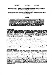
Figure 1: ECHO-G temperature anomalies for scenario A1B, B1 and PIcntrl (pre-industrial control run) with observations (reference 18801920)
model consists of the ECHAM4 (Roeckner et al., 1996) atmosphere GCM and the HOPE-G (Wolff et al., 1997) ocean model. These model runs were part of the 4th assessment report (AR) of the Intergovernmental Panel on Climate Change (IPCC, 2007). The A1B scenario describes a future world of rapid economic growth and global population that peaks in mid-century and slowly declines thereafter while new efficient technologies will then be introduced. CO2 , CH4 , N2 O, N Ox , CO and SO2 concentrations are derived from this economic and demographic scenario. Figure 1 illustrates ECHO-G temperature anomaly projections for different scenarios. These projections show an increase of global temperature by nearly three degrees Kelvin for the A1B scenario compared to present day conditions. The atmospheric resolution of ECHOG is T30 in the horizontal (corresponding to a grid spacing of 3.75◦ ) and 19 layers in the vertical. The oceanic resolution is T42 (2.8◦ ) with a meridional refinement up to 0.5◦ in the tropics and 20 vertical layers.
3
Variations of ∆LOD
Angular momentum fluctuations in the various components of the Earth (so-called subsystems) are reflected by temporal variations of Earth rotation. The solid Earth’s reaction on the redistributions and motions of masses follows from the
law of angular momentum conservation within a closed system: ~ = I~ L ω + ~h.
(1)
The error of ∆LOD due to this approximation is in the order of 10−16 s and is negligible. The relation between the variations |~ ω (t)| and length-of-day changes follows from the definition of ∆LOD, as the duration of one revolution of the Earth reduced by 86400 s:
In this equation I denotes the combined tensor of inertia of the solid Earth and its fluid subsystems, ~h stands for angular momenta with respect to the reference frame (so-called relative ~ on the left angular momenta) and the vector L hand side denotes the total angular momentum of the whole system. The Earth rotation vector is denoted by ~ ω . If external torques due to the gravitational influence of Sun and Moon are neglected, the Earth can be viewed as a closed system. Equation 1 is a simplification of the wellknown Liouville differential equation (Lambeck, 1980). It is valid on condition of two assumptions: First, the Earth rotation vector and the angular momentum vector ~h are considered to be parallel. Second, the tensor of inertia is assumed to be rotationally symmetric with respect to the rotation axis of the Earth. Since both assumptions are not perfectly fulfilled, the orientation of the Earth rotation vector changes with respect to an Earth-fixed reference frame (polar motion) which is not subject of this paper. For studies on ∆LOD these effects are minor (H¨opfner, 1996). Variations of Earth rotation are computed with respect to a uniformly rotating geocentric reference frame with its z-axis, about which it rotates, pointing approximately to the direction of the maximum moment of inertia. The angular velocity of the uniform rotation is one revolution per sidereal day: Ω = 2π/86164s−1 . Due to geophysical processes and gravitational torques this uniform rotation is slightly disturbed and the Earth rotation vector can be written as m1 (t) ω ~ (t) = Ω · m2 (t) , mi ≪ 1 . (2) 1 + m3 (t)
where Cm is the polar moment of inertia of the Earth’s crust and mantle. Polar motion is related to the temporal variation of m1 (t) and m2 (t). Equations 3 and 4 show the dependance of ∆LOD(t) on m3 (t). In the following we will focus on atmospheric effects on length-of-day changes. As mentioned above, it is well known that the largest part of observed variations of ∆LOD on time scales from months to a few years is caused by changes in axial relative atmospheric angular momentum hAAM due to zonal wind variations (Gross et al., z 2004):
The dimensionless quantities mi denote small disturbances of the uniform rotation (Munk and McDonald, 1960). Fluctuations of the angular velocity of the Earth are equivalent to changes of length-of-day (∆LOD). They follow from temporal variations of the absolute value of the Earth rotation vector |~ ω(t)|, which are computed by q |~ ω (t)| = Ω m1 (t)2 + m2 (t)2 + (1 + m3 (t))2
4
≈ Ω(1 + m3 (t))
(3)
∆LOD(t) =
2π − 86400 s . |~ω (t)|
(4)
When higher order terms, external torques and temporal changes in the tensor of inertia are neglected, the insertion of Equation 2 into Equation 1 yields for the third component (Gross et al., 2004) m3 (t) = −∆hz (t)/ΩCm
hAAM z hAAM z
= =
Z
ρr2 (r × v)z dV
r g
Z Z
Vatm 3 Z
η
λ
(5)
(6)
ps ucos2 ϕdϕdλdη (7) ϕ
Equation 7 shows the global mass integration over the atmosphere expressed in spherical coordinates. In the horizontal plane the integration is done over ϕ (latitude) and λ (longitude). Zonal windspeed u and surface pressure ps are obtained from the model’s output. η is the standardized vertical coordinate of the atmospheric GCM. Boundaries of η are 0 for the top of the atmosphere and 1 for the Earth’s surface.
Results
From the ECHAM5 simulations a 2m-temperature anomaly time series has been derived. Since the simulation is driven by observed or reconstructed SSTs and SICs, temperature values over the ocean were excluded
0
axial AAM in SI-units
observed ∆ lod
∆lod (in s)
-1.0e-03
8.0e+25 9.0e+25 1.0e+26 1.1e+26 1.2e+26 1.3e+26 1.4e+26 1.5e+26
compared sim. axial AAM and lod time series simulated axial AAM 1.0e-03
because they are highly affected by the SST. Therefore a high correlation with an observed temperature time series would not necessarily demonstrate any model skill. In Figure 2 the three ensemble members are represented by the dashed lines. The correlation with the observed temperatures is very high even though data points over the ocean have been excluded. The dashed lines show a fairly small spread which indicates a small model uncertainty. The solid bold line (observations) is right in between the dashed lines during many time intervals suggesting that the simulations are quite realistic.
1970
1980
1990
2000
year
Figure 3: Time series of simulated axial AAM and ∆LOD (7yr running mean removed)
global 2m-temperature anomaly over land
and semi-annual cycle but also El Ni˜ no peaks (e.g., 1983) are well reconstructed. A fingerprint of this typical oscillation can be found in the wavelet spectrum of the simulated AAM (Figure 4) where a lot of energy is apparent in a broad band with periods from three to six years.
ensemble member
-0.5
temperature (in K) 0 0.5
observed
8
1
Wavelet power spectrum of simulated axial AAM
1940
1960
1980
2000
period (in years)
0.5
From the atmospheric simulations the global axial AAM is calculated by the integration shown in Equation 7. The model is discretising zonal windspeed on 31 model levels (η-levels). To avoid interpolation through mountains the vertical integration is done over these hybrid η-levels. In contrast to pressure levels the η-levels follow the terrain and are by definition above surface. Integrations over pressure levels tend to overestimate global axial AAM. The simulated AAM time series are plotted together with observed ∆LOD variations from the IERS C04 series in Figure 3. Decadal changes due to core-mantle-interaction have been removed from the observations by substracting a seven year running mean. The effect of longperiodic tides has been removed by filtering. Short periodic tide effects are purged by only considering monthly mean values. The remaining signal is highly correlated with the axial relative AAM time series. Not only the annual
0.25
Figure 2: Simulated ECHAM 5 2m-temperature anomalies for 20th century (reference 1961 to 1990)
4
year
0
1920
2
1900
1
1880
1970
1980
1990
2000
year
Figure 4: Wavelet power spectrum of sim. axial AAM (period 1962 to 2003) The ECHO-G scenario runs show a strong trend in the axial AAM (Figure 5). Under this A1B climate change scenario the atmosphere induces an increased global AAM. By the year 2100 the increase amounts to 10 percent compared to the 2001-2010 mean. In Figure 6 trends of zonal windspeeds at 300 hPa are displayed. Southern Hemisphere jet stream gets strengthened. In the Northern Hemisphere the region of strongest trends is the Northeast Atlantic. Generally trends over land are weaker. This change pattern is in good consistency with the results of former studies (e.g.,
Lorenz and DeWeaver, 2007).
Figure 5: Time series of global axial AAM (5 yr running mean) ECHO-G A1B scenario In the year 2100 the increased axial AAM would cause a lengthening of a solar day by about 0.65 ms. An integration of the computed ∆LOD values over the whole 21st century leads to the prediction that the Earth will be about 11.86 s behind schedule by 2100. However it should be kept in mind that this result comprehends solely the effect of the atmospheric motion term which is superimposed by other effects. For instance the slowing of Earth rotation due to the loss of angular momentum to the moon will lead to an additional delay of 40 s until the year 2100.
Figure 6: Zonal windspeed trends at 300hPa for 21st century from ECHO-G A1B runs (ensemble mean), shaded areas have no significant trend)
5
Discussion
The ECHAM5 simulations of atmospheric winddriven effects on ∆LOD appear to be very realistic since the 2m-temperature profiles of the ensemble members show little departure from each other and agree well with observations. The well
reproduced global temperature anomaly time series is also pointing at realistic circulation patterns. Since axial AAM explains more than 80 percent of the variance of ∆LOD on interseasonal and interannual time scales (Gross et al., 2004), the derived ∆LOD series looks very reasonable, too. Not only characteristics in the frequency domain but also amplitudes of the simulated axial AAM are very well captured and exceed results of previous low resolution GCM studies in quality. Improvements in the models have been achieved in the representation of the orography due to higher horizontal resolution which should produce more realistic winds in mountainous regions. Furthermore simulated winds at the tropopause may have large absolute errors due to large magnitudes and due to a rudimentary treatment of the stratosphere in the previous models. Obviously higher model resolution tends to produce more realistic results. This is not trivial since we are dealing with axial AAM, i.e. a globally integrated variable (Stuck, 2002). ECHO-G A1B scenario runs show a very strong century-long increase in AAM. The dynamic reason of the increase cannot be retraced easily. Strongly increased temperatures in the upper tropics enhance the meridional temperature gradient. In the inner tropics the tropopause level is rising. Therefore the tropopause slope towards the poles is getting intensified. Stratospheric cooling and tropospheric warming amplify the meridional temperature gradient. Due to thermal wind balance westerlies become stronger. The increase in kinetic energy at the tropopause level is consistent with the rise in tropopause height because synoptic waves are trapped in the troposphere (Lorenz and DeWeaver, 2007). This does not contradict the popular impression that the Arctic is especially warming, as the Arctic warming is primarily confined to the very near surface levels. For validation purpose one should compare results to other state-of-the-art models. Abarca del Rio (1999) found trends in reanalysis data which explain an increase in ∆LOD of about 0.5 ms/century during the last 50 to 60 years. The amplitude of zonal windspeed trends for the 21st century seems to be very strong in the ECHO-G runs compared with other model results. Consequently the predicted change in ∆LOD of about 0.65 ms/century is significantly higher than the value of 0.181 ms/century which was derived
from an CMIP2 (Meehl et al., 2000) model ensemble in the analysis of de Viron et al. (2002) even though the increase in CO2 (1% per year) is higher compared to the A1B-scenario (∼0.6% per year). In the CMIP2 study the HadCM2 model reached 0.53 ms/century. This shows that the uncertainty of models is a big issue. On interdecadal time scales other effects become more dominant and cannot be neglected (de Viron et al., 2002). Among those are the angular momentum loss to the sun and moon due to tidal friction (2 ms/century), sea level rise (0.05 ms/century), core motion 0.1-0.2 ms/century and the pressure term of the atmosphere (-0.075 ms/century). Nevertheless axial AAM changes will play a key role in future LOD variations.
6
Acknowledgements
This paper was developed within a project supported by DFG grants HE 1916/9-1 and DR 143/12. The authors thank the Deutsches Klimarechenzentrum (DKRZ), Hamburg, Germany, for providing the CPU time for the standalone runs, the Hadley Centre for providing the SST/SIC data and the IERS for providing the C04 time series.
7
References
Abarca del Rio, R.: The influence of global warming in Earth rotation speed. Ann. Geophys., 17, 806-811, 1999. de Viron, O., V. Dehant, H. Goosse, and M. Crucifix: Effect of global warming on the length-ofday. Geophysical Research Letters, VOL. 29, NO. 7, 10.1029/2001GL013672, 2002. Fr¨ ohlich, C. and J. Lean: The Sun’s total irradiance: Cycles, trends, and related climate change uncertainties since 1976, Geophysical Research Letters 25(23), 4377, 1998. Gross, R.S., I. Fukumori, D. Menemenlis, and P. Gegout: Atmospheric and oceanic excitation of length-of-day variations during 1980-2000. J. Geophys. Res., 109, B01406, doi:10.1029/2003JB002432, 2004. Hide, R.: Interaction between the Earth’s Liquid Core and Solid Mantle. Nature 222, 1055 - 1056; doi:10.1038/2221055a0, 1969. H¨ opfner, J.: Seasonal oscillations in length-of-day. Scientific Technical Report, No.: STR96/03, 1996. IPCC: Climate Change 2007: The Physical Science Basis. Intergovernmental Panel on Climate Change, http : //www.ipcc.ch/ipccreports/ar4 − wg1.htm, 2007. Lambeck, K.: The Earth’s Variable Rotation: Geophysical Causes and Consequences. Cambridge University Press, New York, 1980.
Legutke, S. and Voss, R.: The Hamburg AtmosphereOcean Coupled Circulation Model ECHO-G. Technical Report No. 18, German Clim. Comput. Cent., Hamburg, Germany, 1999. Lorenz, D. J., and E. T. DeWeaver: Tropopause height and zonal wind response to global warming in the IPCC scenario integrations, J. Geophys. Res., 112, D10119, doi:10.1029/2006JD008087. 2007. Meehl, G. A., G. J. Boer, C. Covey, M. Latif, and R. J. Stouffer: The Coupled Model Intercomparison Project (CMIP), Bull. Amer. Meteorol. Soc., 81, 313 318, 2000. Min, S.-K., S. Legutke, A. Hense, and W.-T. Kwon: Internal variability in a 1000-year control simulation with the coupled climate model ECHO-G - I. Near-surface temperature, precipitation and mean sea level pressure. Tellus, 57A, 605-621. 2005. Min, S.-K., S. Legutke, A. Hense, U. Cubasch, W.-T. Kwon, J.-H. Oh, and U. Schlese: East Asian climate change in the 21st century as simulated by the coupled climate model ECHO-G under IPCC SRES scenarios. J. Meteor. Soc. Japan., 84, 1-26. 2006. Munk, W.H. and MacDonald, G.J.F.: The rotation of the Earth: A geophysical discussion. Cambridge University Press, New York, 1960. Rayner, N.A., P. Brohan, D.E. Parker, C.F. Folland, J.J. Kennedy, M. Vanicek, T. Ansell and S.F.B. Tett: Improved analyses of changes and uncertainties in sea surface temperature measured in situ since the midnineteenth century: the HadSST2 data set. Journal of Climate.19(3) pp. 446-469. 2006. Roeckner, E., K. Arpe, L. Bengtsson, M. Christoph, M. Claussen, L. Dmenil, M. Esch, M. Giorgetta, U. Schlese and U. Schulzweida: The atmospheric general circulation model ECHAM-4: Model description and simulation of present-day climate, Rep. 218, Max-Planck-Institute (MPI) for Meteorology, Hamburg, Germany, 1996. Roeckner, E., G. Buml, L. Bonaventura, R. Brokopf, M. Esch, M. Giorgetta, S. Hagemann, I. Kirchner, L. Kornblueh, E. Manzini, A. Rhodin, U. Schlese, U. Schultzweida und A. Tompkins: The atmospheric general circulation model ECHAM 5. PART I: Model description, Rep. 349, MPI for Meteorology, Hamburg, Germany, 2003. Stuck, J.: Die simulierte axiale atmosph¨ arische Drehimpulsbilanz des ECHAM3-T21 GCM, PhD thesis, Bonner Meteorologische Abhandlungen, 56, Asgard, Sankt Augustin, 2002. Taylor, K.E., D. Williamson and F. Zwiers: The sea surface temperature and sea-ice concentration boundary conditions of AMIP II simulations. PCMDI report No. 60, 20 pp, 2000. Wolff, J. O., E. Meier-Reimer and S. Legutke: The Hamburg ocean primitive equation model, DKRZ 13, 98 pp., German Clim. Comput. Cent., Hamburg, Germany, 1997.