SIMULATION OF MULTIPACTOR EFFECT THROUGH THE INDIVIDUAL SIMULATION OF ELECTRONS F. Pérez(1), J. de Lara(1), L. Galán(2), M. Alfonseca(1), I. Montero(3), E. Román(3), D. Raboso(4) (1)
Escuela Técnica Superior de Informática, Universidad Autónoma de Madrid Francisco Tomás y Valiente 11, 28049-Madrid, Spain Email: {francisco.perez, juan.delara, manuel.alfonseca}@uam.es (2)
Departamento de Física Aplicada, Universidad Autónoma de Madrid 28049-Madrid, Spain Email:
[email protected] (3)
Instituto de Ciencia de Materiales de Madrid, CSIC 28049-Madrid, Spain Email: {imontero, eroman}@icmm.csic.es (4)
ESA/ ESTEC Keplerlaan 1, 2200 AG Noordwijk, The Netherlands Email:
[email protected] ABSTRACT In the context of the ESA Program AO 4025 Surface Treatment and Coating, we have developed a simulator called MEST for the prediction of the multipactor effect. The simulator has been developed using a micro level object-oriented approach, where each electron in the simulation is an independent object. This approach differs from other models described in the literature, which are macro level or intermediate, handling electrons in packages rather than individually. MEST works with a simplified model of a waveguide, where a radiofrequency potential is applied to the plates. The space between the plates is assumed to be a vacuum, except for the presence of a number of free electrons. The individual trajectories of all the electrons in the RF field are computed, although no space charge effects are assumed. When electrons collide with the plates, secondary emission of electrons is simulated. The secondary electron emission yield (SEY) is computed with a detailed Monte Carlo model, which has been validated using experimental data. It depends on the surface material (bulk), but also on surface finish properties, such as air contamination, cleanliness or surface treatments. If certain conditions hold, the number of electrons between the plates may increase out of control, until a multipactor discharge occurs and the waveguide becomes unusable. The object of the simulator is to predict the occurrence (or not) of this phenomenon for different surface materials. The simulator has been validated using experimental data from ESTEC (ESA), UAM and TESAT. Several materials have been tested. The results show good agreement with the experimental data. 1. INTRODUCTION The multipactor effect [5][10] is a spurious discharge that may take place in a waveguide as a consequence of the electron avalanche produced when secondary electrons, ripped away from the inner walls of the waveguide by the impact of free electrons, resonate with the electric field transmitted by the waveguide. The continual increase of the number of electrons in the vacuum filling the waveguide may give rise to a discharge which makes the waveguide unusable. In order to protect the waveguide, different material coatings have been tested with the aim of reducing the secondary emission of the walls. The effect usually appears in the sections where the waveguide calibre is smallest, such as filters placed inside the waveguide to control its impedance and its frequency response properties. Multipactor experiments are relatively expensive, time and resource consuming. Thus, with appropriate models of the phenomena and if the different materials can be characterized, simulation can be a valuable tool for selecting the most promising materials. We have developed the software tool MEST (Multipactor Electron Simulation Tool), which performs simulations by tracking each electron individually. We follow a discrete-event approach [6], where the events are the collisions of electrons with the waveguide walls. The simulator generates V-f·d maps of the multipactor discharge detected in the simulations. Materials are described either using the usual parameter set (E1, E2 and σmax), or by a more detailed model, where the contributions due to true secondary, backscattered or elastically reflected electrons are given their own sets of
parameters, together with additional parameters for the angle dependence. This paper has been organized as follows. Section 2 gives an overview of the model for the SEY which we have used. Section 3 explains our discrete-event simulation procedure. Section 4 presents the main characteristics of the software. Section 5 shows results obtained for some materials. Finally, section 6 ends with the conclusions. 2. THE SECONDARY EMISSION MODEL In this section we give an overview of the Secondary Emission Yield (SEY) model we use in the software. For further details, the reader can consult [3]. When an electron collides with one of the plates, it can be absorbed, elastically or inelastically backscattered, or a number of true secondary electrons may be generated. The three kinds of emitted electrons provide their own contributions to the SEY curve, which is a function of the impacting energy (Ep) and the incidence electron angle (ϕ). The addition of the three contributions results in the total SEY, which also depends on the material, and on surface finish properties, such as air contamination, cleanliness or surface treatments. The SEY value for an impact at a certain energy and angle gives the average number of generated electrons. Fig. 1 shows a typical SEY curve for a normal incidence angle. This curve is usually modelled by three magnitudes: E1 and E2 are the energies when the SEY value is 1, Emax is the energy where the SEY gets its maximum value. We use a model with a more refined set of parameters, which result from fitting experimental data for many materials, either from our experimental data or from the literature, mostly from [9].
Fig. 1. A Typical SEY Curve Thus, the total SEY (σ), is modelled as the sum of the contributions of inelastically backscattered electrons (η), elastically backscattered electrons (ε), and true secondary electrons (δ): σ(Ep) = η (Ep)+ ε(Ep)+ δ(Ep), where ε, δ and η are dependant on material properties, in particular η depends also on the atomic number of the coating material. Additionally, we have to take into account the angle ϕ with which the electron collides. This can be separately modelled as for each type of collision. In this way, the final SEY has an expression like the following: σ(Ep, ϕ) = η (Ep, ϕ)+ ε(Ep, ϕ)+ δ(Ep, ϕ). When an electron impacts a plate, the probability for each kind of emission is thus given by: Pe (E p , ϕ ) = ε (E p , ϕ )
Pb (E p , ϕ ) = η (E p , ϕ )
Ps (E p , ϕ ) = 1 − Pe (E p , ϕ ) − Pb (E p , ϕ )
The probabilities of a collision producing elastic or inelastically backscattered electrons are Pe(Ep,ϕ) and Pb(Ep,ϕ), respectively. Both collisions produce one emitted electron. In the true secondary emission case, with probability Ps(Ep,ϕ), a random number of electrons n are produced. These are generated with a probability Pn(Ep,ϕ), which has a Poisson distribution [3]. Once the number of true secondary electrons has been obtained, their energy is sequentially computed by an inverse cumulative probability function. By the energy conservation principle, the total energy of the output electrons is equal or less than the energy of the impacting electron. Finally, the output electrons emission angles are calculated. We consider emission angles θ, with respect to the inward
normal to the xy plane, and ζ in the xy plane. If the output electron is elastically or inelastically backscattered, its output angles are the same as its input angles (it is perfectly reflected). In the case of a true secondary electron, the angles are calculated using the cosine law distribution. 3. THE MULTIPACTOR SIMULATION For the simulation, we have used a typical discrete-event procedure, using the “event scheduling” approach [6]. In this kind of simulation, time advance is driven by the occurrence of the events. When an event occurs, the system state changes and new events can be scheduled to occur in the future. For the simulation, the main idea is to have an event queue, ordered by the time at which the event should be processed. In our case, the events are the impacts of the different electrons with the plates. The collision time can be efficiently calculated, because in the case of parallel plates geometry, we can analytically compute solutions to the electron trajectories. In this way, when an electron collides with a plate, we schedule a new event calculating the time of its next collision. The simulator loops through all the events in the queue, advancing the simulation time, generating new events (new collisions) and placing them in time order in the queue. Each electron is individually modelled as an object in the object-oriented paradigm [1], with the capability to compute the time of its next collision and thus schedule new collision events. Each collision event has a link to the electron that generated it. Figure 2 shows the control graph of the simulation procedure. Initially, a population of electrons is generated. Each electron is given a normally distributed energy. All start at one of the plates. Moreover, they are assumed to have impacted that plate at a random time in the first period of the electromagnetic field. In this way, this collision initial time is used to initialize the event queue. Then the main simulation loop begins. The simulator takes the first event in the queue, and the associated electron. It calculates the type of collision using the model of the previous section. For each newly generated electron in the collision, it calculates the next impact time and schedules new events. Here, absorption may occur, thus no new event is generated and the electron is deleted from the simulation. The simulation ends when a final condition is met (multipactor appears, does not happen, or a certain number of cycles is reached). The final conditions are discussed in the next section.
Fig. 2. A Scheme of the Simulation Procedure 4. THE SOFTWARE We have implemented the previous concepts in the software tool MEST. The software runs in the Windows operating system. Fig. 3 shows its main window.
Optimization parameters for border seek
Configuration of initial electron population
Run-time information
Accuracy of V-f·d map Geometry configuration
Simulation results for each gap and voltage
RF Field configuration
Final Conditions for the simulation
Fig. 3. The Main Window of MEST In the main window, it is possible to set the experiment initial and final conditions, to prepare sets of experiments and to visualize run-time information when a simulation is running. The initial conditions of the experiment include the number of initial electrons and their initial energy. This is given as a normal distribution, for which the average and dispersion is needed. As all the initial electrons start at one of the plates, it is possible to specify the starting incidence angle of the electron population as a normal distribution. There are two kinds of geometry supported by MEST: infinite and finite parallel plates. For the first case, it is possible to specify a height (a gap). For the second kind, a width and a length should also be specified. Finally, in order to configure an experiment, the electromagnetic field need to be specified giving the voltage and frequency. It is possible to prepare sets of experiments, which will trigger a number of simulations, one for each experiment. This can be done by specifying a range of gap values and/or voltage values. A simulation is then performed for each combination of gap and voltage. The ranges are specified by giving the minimum and maximum values, as well as their increment.
Fig. 4. Specifying the SEY Properties of Alodine. The properties of the materials also need to be specified. They can be given using the usual parameter set E1, E2 and σmax, or a more refined set of parameters [3]. Fig. 4 shows the specification for a certain measure of Alodine. Once the parameters have been set, the SEY curve can be obtained in a separate window. The goal of the simulation is to signal the appearance or not of multipactor given the initial conditions. The conditions under which a simulation stops can also be defined. For this purpose, a quantity N is given, in such a way that, when the
current number of electrons in the simulation is greater than N times the initial number, the simulation stops predicting a multipactor occurrence. Conversely, if the number of electrons reaches 1/N times the initial number, the simulation stops giving a no multipactor prediction. Note that choosing the right N is crucial here. A low value of N could make the simulation stop with a multipactor prediction when a spurious increase of electrons occurs (see the discussion in next subsection). On the other hand, a high value of N results in longer simulations. In addition, it is possible to set a maximum number of cycles for the simulation. 4.1 Simulation Outputs MEST produces several output forms during the simulation. The first one is the evolution of the number of electrons. Two examples are shown in Fig. 5. In the one to the left (a), it can be seen how the number of electrons decreases every 1.5 cycles approximately. Note also that, although the population increases at first, at the end, the electrons tend to be absorbed, thus no multipactor occurs. The cycle height is bounded by the maximum SEY of the material, as this is the maximum number of electrons ripped at each collision. Therefore, a correct final condition for the simulation has to be greater than the maximum SEY, which is dependent on the material. In the figure to the right, multipactor occurs. It can be seen how, after a transitory period, the population increases with a period of 3.5 cycles approximately. Note also that, if a lower final condition had been set, the simulation would have been given a “no-multipactor” due to the initial transitory period, in which some electrons where absorbed.
(a) (b) Fig. 5. Evolution of the Number of Electrons in a Simulation (a) No Multipactor, (b) Multipactor. Another output window shows an animation with the electron trajectories during the simulation. This output form is also calculated and shown during the simulation. Fig. 6 depicts a moment in a simulation for Alodine with finite parallel plates geometry. The colour of the electrons reflects the number of collisions they have had during the simulation. The colour scale goes from black (new ripped out electron) to red (over ten collisions).
Fig. 6. Animation of the Electron Trajectories, Finite Parallel Plates geometry. The main output form of MEST is a V – f·d map. This is a two-dimensional graphic showing the results (positive or
negative prediction of multipactor occurrance) of a set of simulations. Fig. 8a shows an example of this output form for Alodine. Each point in the map is a simulation. The colour of the point means occurrence (red) or not (blue) of multipactor. In addition, we assign a colour range for multipactor, which quantitatively shows how fast the multipactor or the absorption occurred. Red means a very strong multipactor effect, while orange means a weaker multipactor (it took more time to appear). In a similar way, blue means a quick absorption of the electrons, while green means that the absorption took more time.
(a) (b) Fig. 8. A V – f d Map for Alodine (a) and Multipactor Modes (b) In order to reduce the number of experiments needed to obtain the V – f·d map (thus reducing the overall computing time), it is possible to use an algorithm to search for the borders of the curve (see Fig. 3). In this way, the algorithm starts triggering the corresponding simulations from left (lower gap) to right (higher gaps), and from the lowest specified Voltage. When a simulation gives absorption and the next one results in multipactor, a left border has been found. The user can specify a number of refinements which give a higher accuracy. In this way, the gap increment is halved progressively and new experiments are launched. The accuracy in Voltage and gap is also estimated and presented to the user (see Fig. 3). Once the left border (for a given Voltage) has been found, the right border is sought, starting from right to left. After this, the Voltage is increased and the procedure is repeated. Note also that the refinements also work with the Voltage. This algorithm reduces the number of experiments, as the simulations of the inner points in the susceptibility curve are not performed. A similar output form shows the modes [8] of the electrons. These are the integer numbers of RF periods an electron takes to go from one impact to the next, plus one. Thus, mode 1 is just a semi-period, as it is the minimum time an electron takes to go from one side of the geometry to the other. Fig. 8b shows the modes for a simulation with Alodine (the first nine modes are shown). Other, higher modes may occur at higher voltages, but the simulation stopped at 3000 Volts. Note how the Hatch and Williams theory predicts a sharp edge at the lowest-left end of the curve (in mode 1). In all our simulations, the curve is rounded. This result seems to be validated by experimental data [12]. Note how this output form cannot be obtained if we use the optimization algorithm, as most multipactor experiments inside the curve are not performed. 5. RESULTS FOR SOME MATERIALS The aim of the development of this simulator was to test the feasibility, for different types of surface coatings, of reducing the occurrence of multipactor by diminishing the SEY of the material. In this section, we show some simulation results for different materials.
Fig. 9. Simulation Results for (left-to-right and top-to-bottom) Aluminium, Copper, Alodine, Titanium Nitride, Gold over Chromated Anomag (bad quality), Gold over Chromated Anomag (good quality) Notice that the results for the Alodine experiment in Fig. 9 are worse than those we showed in Figure 8, due to factors like air exposure, roughness and oxidation. Also, in Fig. 9, we show two simulations for Anomag. The SEY data for each experiment have been measured from two different samples. The different external conditions in which both samples were measured and manipulated have made a variation of more than 300 Volts in the lower part of the susceptibility curve.
6. CONCLUSIONS In this paper we have presented MEST, a software for the prediction of the multipactor effect. The software uses a detailed model of the SEY and uses a discrete-event simulation procedure where each electron is individually tracked. This approach is different of other models described in the literature [4][7][11], which are macro level or intermediate, handling electrons in packages rather than individually. The software offers a number of graphical outputs that help in the simulation planning, results analysis and understanding. The results for some materials obtained with MEST show good agreement with experimental data. One must take into account, however, that the conditions of the materials change their SEY properties, which means that the simulation results in a given case can differ from those shown in Fig. 9. REFERENCES [1] Booch, G. “Object Oriented Design”. Benjamin-Cummings, 1991. [2] Cimino, R., Collins, I. R., Furman, M. A., Pivi, M., Ruggiero, F., Rumolo, G., Zimmermann, F. “Can Low-Enery Electrons Affect High-Energy Physics Accelerators?”. Phys. Rev. Lett., Vol. 93, p. 014801, 2004 [3] de Lara, J., Pérez, F., Alfonseca, M., Galán, L., Raboso, D. “Multipactor Electron Simulation Tool (MEST)”, Proc. 26th IEEE Int. Power Modulator Symposium and 2004 High Voltage Workshop, pp.: 547-550 [4] Devaz, G. “Multipactor simulations in superconducting cavities and plasma couplers”, Phys. Rev. Special Topics Accelerators and Beams. Vol. 4, p. 012001, 2001 [5] Farnsworth, P. T. “Television by electron image scanning”. J Franklin Inst., vol. 218, pp.: 411-444, 1934. [6] Fishman, G. “Discrete Event Simulation. Modeling, Programming and Analysis”. Springer Series in Operations Research. 2001. [7] Galán, L., Jiménez, M. A., Rueda, F. "Development of a computer model for the multipactor effect". ESA-ESTEC Contract 6577/85/NL/PB 1990/Rider, ESA, 1991. [8] Hatch, A. J., Williams, H. B. 1954. "The Secondary Electron Resonance of Low-Pressure High-Frequency Gas Breakdown". Journal of Applied Physics, Vol 25, Num 4, April 1954. [9] Reimer, L. “Scanning Electron Microscopy. Physics of Image Formation and Microanalysis”. Springer Series in Optical Sciences 45, Springer-V (1985), chapter 4. [10] Vaugham, J. R. M. “Multipactor”. IEEE Transactions on Electron Devices, Vol 35(7), pp.: 1172-1180, July 1988. [11] Vender, D., Smith, H.B., Boswell, R. W. “Simulations of multipactor-assisted breakdown in radio frequency plasmas”. J. Apply. Phys., Vol. 80, p. 4292, 1996. [12] See for example data of Woo for Al in: Woo, NASA report No. 32-1500; also reproduced in [13] Fig.3.3.3 pp.: 2627. [13] Woode A., and Petit, J. Estec Working Paper No. 1556. “Diagnostic Investigations into the Multipactor Effect, Susceptibility Zone Measurements and Parameters Affecting a Discharge”, ESTEC, Noordwijk, 1989.