IEEE TRANSACTIONS ON GEOSCIENCE AND REMOTE SENSING, VOL. 53, NO. 4, APRIL 2015
1921
Simulation of the SMAP Data Stream From SMAPEx Field Campaigns in Australia Xiaoling Wu, Jeffrey P. Walker, Christoph Rüdiger, Member, IEEE, Rocco Panciera, and Douglas A. Gray
Abstract—NASA’s Soil Moisture Active Passive (SMAP) mission will provide a ∼10-km resolution global soil moisture product with a 2–3-day revisit by exploiting the synergy between active and passive observations. However, soil moisture downscaling techniques required to exploit this synergy have not yet received extensive testing, being limited to mostly synthetic data. Consequently, airborne field campaigns such as the SMAP Experiments (SMAPEx) have been designed to provide experimental data to fill this gap. The objective of this study is to assess the reliability of SMAP prototype data stream derived from airborne observations, with the aim of providing a simulated SMAP data set for prelaunch algorithm development of SMAP. Specifically, the reliability of incidence-angle normalization and spatial resolution aggregation for airborne observations was assessed for this purpose. The impact of azimuthal angle on active–passive observations was analyzed to assess the potential influence of SMAP rotating antenna on observations. Results showed that the accuracies of angle normalization were ∼0.8 dB for active and 2.4 K for the passive observations (1-km resolution), while the uncertainties associated with spatial upscaling were 2.7 dB (150-m resolution) and 2 K (1-km resolution). Although azimuthal signatures associated with the variable orientation of surface features were observed in the high-resolution observations, these tended to be smoothed when aggregating to coarser resolution. As these errors are expected to decrease further at the coarser resolution of SMAP, results suggested that data from SMAPEx can be reliably used to simulate SMAP data for subsequent use in active–passive soil moisture algorithm development. Index Terms—Active microwave, azimuth effect, incidenceangle normalization, passive microwave, Soil Moisture Active Passive (SMAP), Soil Moisture Active Passive Experiments (SMAPEx), spatial scaling.
I. I NTRODUCTION
G
LOBAL measurements of soil moisture are vital for understanding the global water, energy, and carbon cycles, which have a significant impact on agriculture, hydrology, and
Manuscript received October 21, 2013; revised April 9, 2014 and June 19, 2014; accepted July 21, 2014. The SMAPEx field campaigns were supported by Australian Research Council Discovery (DP0984586) and Infrastructure (LE0453434 and LE0882509) grants. X. Wu, J. P. Walker, and C. Rüdiger are with the Department of Civil Engineering, Monash University, Clayton, Vic. 3800, Australia (e-mail: xiaoling.
[email protected];
[email protected];
[email protected]). R. Panciera is with the Cooperative Research Centre for Spatial Information, The University of Melbourne, Carlton, Vic. 3053, Australia (e-mail:
[email protected]). D. A. Gray is with the School of Electrical and Electronic Engineering, The University of Adelaide, Adelaide, SA 5005, Australia (e-mail: douglas.gray@ adelaide.edu.au). Color versions of one or more of the figures in this paper are available online at http://ieeexplore.ieee.org. Digital Object Identifier 10.1109/TGRS.2014.2350988
meteorology [1]. However, accurate estimation of soil moisture is currently hampered by a general lack of in situ soil moisture observations. Even when available, in situ soil moisture measurements are often spatially and temporally too sparse to be used in studying the impact on important meteorological phenomena in the surface and atmospheric boundary layers [2]. Moreover, soil moisture exhibits large spatial and temporal fluctuations due to the high spatial variation of rainfall patterns, vegetation distribution, soil texture, and topography. The resulting variability in soil moisture is difficult to characterize with the current sparse in situ networks. Due to the general infeasibility of operating a large in situ soil moisture monitoring network at the required scale, important developments in the retrieval of soil moisture from satellite-based remote sensing have taken place [3], [4]. With recent technological advances in remote sensing [5], soil moisture mapping is becoming more cost-effective over large areas, including at the global scale, providing an important alternative to traditional monitoring using in situ networks or individual point measurements. Consequently, methods are being developed to make use of this emerging soil moisture information to constrain numerical model prediction of soil moisture [6] and hence improve the forecasting of weather, floods, and agriculture-related applications. However, current generation passive microwave remote sensing techniques are not yet able to provide remotely sensed soil moisture data at spatial resolutions better than about 40 km. Microwave techniques (active and passive) have been adopted as the preferred approach due to their more direct link to soil moisture (through the dielectric constant) than optical and thermal techniques. Moreover, passive microwave has the advantage of being less affected by vegetation and roughness with respect to active microwave sensing but suffers from its low spatial resolution [7]–[9]. Studies on soil moisture remote sensing using passive microwave techniques have demonstrated the superiority of the low-frequency sensors [3], [10], [11], with the conclusion that the emission at ∼1.4 GHz is definitely related to the soil moisture due to the reduced interference by the atmosphere, surface roughness and vegetation, and increased observation depth (∼5 cm). Consequently, the Soil Moisture and Ocean Salinity mission [12] was launched by the European Space Agency in November 2009, as the first-ever satellite dedicated to soil moisture measurement using L-band passive microwave measurements. Despite the strong sensitivity of passive microwave observations to near-surface soil moisture monitoring, the relatively coarse spatial resolution of ∼40 km for a spaceborne radiometer poses significant limitations to regional applications such as
0196-2892 © 2014 IEEE. Personal use is permitted, but republication/redistribution requires IEEE permission. See http://www.ieee.org/publications_standards/publications/rights/index.html for more information.
1922
IEEE TRANSACTIONS ON GEOSCIENCE AND REMOTE SENSING, VOL. 53, NO. 4, APRIL 2015
flood prediction, having a resolution requirement of better than 10 km. It has, in fact, been shown by [13] and [14] that hydrometeorological applications such as precipitation systems, which are generally driven by thermal convection, as well as other applications in hydrologic and atmospheric science, have distinguishing features or significant physical interactions at around the ∼10-km scale. Therefore, availability of a 10-km soil moisture product is expected to enhance our understanding and forecasting capabilities of regional weather systems around the world. Moreover, it is expected to benefit agricultural applications and large watershed or river-basin management activities. While soil moisture information at resolution finer than 10 km can be potentially retrieved by active microwave remote sensing, the observations are less sensitive to changes in soil moisture, due to the confounding effects of vegetation conditions and surface roughness, and the relatively low signal-tonoise ratio of the available sensors [15], which means that such high-resolution soil moisture estimates usually have a much larger uncertainty than coarser resolution passive products. NASA’s Soil Moisture Active Passive (SMAP) mission [16], scheduled to be launched in January 2015, proposes to overcome this scale issue by using fine-scale (3 km) active microwave observations to downscale the coarse-scale (36 km) passive microwave observations to a medium-scale (9 km) resolution. The rationale behind SMAP is that the relationship between active and passive observations may be used to overcome the individual limitations of each observation type, ultimately providing soil moisture data with higher accuracy, as well as at a resolution more suitable for hydrometeorological applications [13], [17]. In preparation for the SMAP launch, suitable algorithms and techniques need to be developed and validated to ensure that an accurate fine-resolution soil moisture product can be operationally produced from combined SMAP radiometer and radar observations. To this end, it is essential that field campaigns with coordinated satellite, airborne, and ground-based data collection be undertaken, giving careful consideration to the diverse data requirements for the range of scientific questions to be addressed. Therefore, some field campaigns have been conducted using active and passive microwave airborne observations to address the scientific requirements pertinent to SMAP. Such campaigns include the Southern Great Plains experiment in OK in 1999 (SGP99) [18], [19], the Soil Moisture Experiment in IA in 2002 (SMEX02) [20]–[22], the Cloud and Land Surface Interaction Campaign in OK in 2007 (CLASIC) [23], [24], the Canadian Experiment for Soil Moisture 2010 (CanEx-SM10) [25], the SMAP Validation Experiments (SMAPVEX2008 and SMAPVEX2012) [26], and the SMAP Experiments (SMAPEx) in Australia in 2010 and 2011. The SMAPEx field campaigns provide the opportunity to evaluate the SMAP active/passive baseline algorithms using data that present with different sets of conditions and land covers. These field campaigns are complementary to the other campaigns in addressing scientific requirements of the SMAP mission, therefore representing a significant contribution to the limited heritage of airborne experiments mentioned previously. During the SMAPEx Experiments, airborne prototype SMAP data were collected together with ground observations
Fig. 1. Overview of the SMAPEx site showing the location of the SMAP pixel sized study site in the township of Yanco, Australia, together with the ground focus areas (YA4, YA7, YC, YD, YB5, and YB7; “Y” refers to Yanco) and different flights.
of soil moisture and ancillary data over an area equivalent to a SMAP radiometer footprint (36 km), with the aim to provide SMAP-type data for the development and validation of algorithms and techniques to estimate near-surface soil moisture from the upcoming SMAP mission. Consequently, the main objective of this paper is to assess the reliability of simulated SMAP data using aircraft observations from the SMAPEx field campaigns. In particular, this paper makes use of flights specifically conducted to assess the reliability of the following: 1) the incidence-angle normalization of airborne data to the SMAP reference incidence angle of 40◦ ; 2) the spatial aggregation of airborne active and passive data to the resolution of SMAP observations; and 3) the impact of different azimuthal view angles on the active and passive data. II. DATA S ET A. Experiment Overview SMAPEx comprises a series of three campaigns undertaken over an approximately one-year timeframe in 2010 and 2011. The SMAPEx study site is a semiarid agricultural and grazing area located in Yanco in the Murrumbidgee River catchment in South-Eastern Australia (−34.67◦ N, −35.01◦ N, 145.97◦ E, 146.36◦ E; see Fig. 1) and forms part of the Murray–Darling basin. A complete description of the SMAPEx study area and monitoring activities can be found in Panciera et al. [27]. The SMAPEx experiments were timed to encompass the seasonal variation in soil moisture and vegetation: SMAPEx-1 was conducted from July 5 to 10, 2010, in the austral winter, SMAPEx-2 was carried out from December 4 to 8, 2010, in the austral summer, and SMAPEx-3 took place from September 4 to 23, 2011, in the austral spring. The SMAPEx project was specifically designed to contribute to the development of radar
WU et al.: SIMULATION OF THE SMAP DATA STREAM FROM SMAPEx FIELD CAMPAIGNS IN AUSTRALIA
and radiometer soil moisture retrieval algorithms for the SMAP mission. While the one-week-long SMAPEx-1 and SMAPEx-2 campaigns were focused on providing data for “snapshot” type algorithms, the three-week-long SMAPEx-3 campaign aimed at collecting a longer data record for the development of time-series and change-detection algorithms. SMAPEx-1 was conducted shortly after the sowing of winter crops, with only the emergent plant phase present in the fields under moderately wet soil moisture conditions. SMAPEx-3 captured the intensive growth phase of winter crops in the study area (essentially wheat, barley, and canola) under moderately dry conditions, while SMAPEx-2 was characterized by moist conditions and near-peak crop biomass. The SMAPEx field site was selected due to its flat topography, widely distributed in situ soil moisture monitoring stations, and representation of soil, vegetation, and land use conditions typical of semiarid environments. The main SMAPEx scientific flights included “regional” flights, covering the 36 km × 38 km area equivalent to a pixel of the SMAP products EASE grid at 35◦ S latitude with a 2–3-day revisit time, and other specific flights, including the following: 1) multiangle flights; 2) multiazimuth flights; and 3) multiresolution flights, conducted specifically to address the reliability of using SMAPEx airborne data as a proxy of future SMAP spaceborne observations, which is the focus of this study. Details of each specific flight can be found in Section II. Apart from the airborne observations, the spatial ground sampling activities were also conducted in six focus areas: YA4, YA7, YB5, YB7, YC, and YD (“Y” refers to Yanco; each area has a size of 2.8 km × 3.1 km), which were distributed across the simulated SMAP radiometer pixel. In the following, YA4 and YA7 will be referred to as simply “YA,” and YB5 and YB7 will be referred to as “YB.” While the YA and YD areas were mainly occupied by the irrigated crop, YB and YC were dominated by grass, so as to provide the opportunity to study the impact of the azimuth and incidence angles of the specific flights on the resulting observations with respect to different land cover conditions. Data collected from ground sampling are used as the ground truth for algorithm calibration and validation. B. Airborne SMAP Simulator The airborne data were collected using a SMAP airborne simulator which allows the simultaneous acquisition of active and passive microwave remote sensing measurements at the same frequency as the SMAP sensor (L-band) but at finer spatial resolution. The airborne simulator (Fig. 2) includes the Polarimetric L-band Multibeam Radiometer (PLMR) and the Polarimetric L-band Imaging Synthetic Aperture Radar (PLIS) which, when used together on the same aircraft, provide active and passive microwave observations similar to the expected SMAP data stream, albeit at different incidence angles and spatial resolutions, as discussed in detail in this section. The main characteristics of the SMAP sensors, PLMR, and PLIS are described in Table I, from which it is noted that the
1923
Fig. 2. Airborne simulator including PLMR and PLIS.
airborne sensors from SMAPEx have the same frequency band as SMAP and the same polarization combinations. PLMR has three fixed beams which do not record over continuous range of incidence angle but at three fixed angles, being 7◦ , 21.5◦ , and 38.5◦ ; the PLIS antennas radiate mainly between 15◦ and 45◦ continuously. In order to closely replicate the SMAP data, both the spatial resolution and incidence angle of the airborne observations need to be adapted. Therefore, the 1-km PLMR brightness temperatures and ∼10-m PLIS backscatter need to be aggregated to 36 and 3 km, respectively. Moreover, both PLMR and PLIS observations need to be normalized to a constant 40◦ incidence angle. In addition, since SMAP will make use of a rotating mesh antenna to provide observations over the entire swath, both the radar and radiometer observations will be observed at a range of azimuthal orientations. Therefore, it will be crucial to understand the potential impact on the observations due to the azimuth viewing angle and how this changes depending on specific surface conditions (e.g., vegetation type and tillage conditions). The accuracy of the PLMR radiometer was assessed against hot (blackbody box) and cold (clear sky) calibration targets before and after each SMAPEx flight, as well with in-flight calibration by low-altitude passes of a water body where water temperature and salinity were measured. The radiometer accuracy was estimated to be better than 0.7 K for H-polarization and 2 K for V-polarization, including system noise and in-flight calibration drift [27]. Calibration of the PLIS radar was performed using a combination of six trihedral passive radar calibrators (PRCs) deployed across-swath in a homogeneous grassy field and a distributed forest target. The calibration targets were imaged each day at both the beginning and end of the scientific monitoring flights to check for a potential calibration drift. After radiometric calibration, the difference between the observed and theoretical PRC cross sections was, on average, 0.93 dB (absolute radiometric accuracy) with a standard deviation (SD) of 0.8-dB relative radiometric accuracy [27]. The repeatability of PLIS flights was also calculated by comparing the start overpass to the end overpass, and the resulting rootmean-square deviation (RMSD) was approximately 0.9 dB at copolarization and 1.4 dB at cross-polarization. The possible influence of calibration accuracy during the SMAP data simulation will be described in the following sections. To this end, the accuracy of PLIS observations can meet the radar measurement accuracy requirement of the SMAP, which is around 1.0 dB
1924
IEEE TRANSACTIONS ON GEOSCIENCE AND REMOTE SENSING, VOL. 53, NO. 4, APRIL 2015
TABLE I C HARACTERISTICS OF THE SMAP S ENSORS , PLMR, AND PLIS
Fig. 3. (a) Multiangle flights conducted during SMAPEx-1 and SMAPEx-2 over cropping area YA and grassland YB, at 3000-m altitude, and multiazimuth flights conducted on one occasion during SMAPEx-2 over cropping area YA and grassland area YC, respectively, at 1500-m altitude. (b) Aerial photographs of two multiazimuth mapping areas (1 km × 1 km) within YA (left) and YC (right) areas, respectively, and layout of the land cover type within YA (1—grass, 2—cotton, 3—maize, and 4—wheat) and land cover type within YC (5—uniform grassland).
at copolarization and 1.5 dB at cross-polarization at 3-km resolution, including the calibration error, contamination terms, and speckle noise. C. Flight Design In order to closely replicate the SMAP data, every portion of the study area should be observed at the same incidence angle of SMAP (40◦ ). However, this is not easily achieved using a small experimental aircraft with airborne instrumentation over an area as large as the SMAPEx study area within the time constraints of the daily sampling. Therefore, multiangle flights [see Fig. 3(a)] were designed to provide data for characterizing the angular variation of brightness temperature and radar backscatter together with reference data observed at 40◦ ± 2.5◦ over portions of the study area. For this testing, data were collected from the SMAPEx-1 and SMAPEx-2 field campaigns. During the SMAPEx-1 field campaign, multiangle flights were conducted on three days: July 6, 8, and 10, 2010. During SMAPEx-2, multiangle flights were performed on December 7, 2010, only, thus allowing evaluation of the normalization
skill robustness under the increased biomass conditions of SMAPEx-2 (full-grown crops). Areas selected as the focus of multiangle flights were within the two SMAPEx target areas YA and YB (a cropping area and a grassland area, respectively), as shown in Fig. 3(a). The flying altitude was around 3 km to collect multiangle active microwave observations at approximately 10-m spatial resolution and passive microwave observations at 1-km resolution. For each flight, two ground strips of radar backscatter (σ ◦ ) were imaged, due to the PLIS configuration, each of approximately 2.2 km in width, together with a radiometer brightness temperature (T b) swath of approximately 6 km in width. Eight adjacent parallel flight lines separated by approximately 360 m were conducted in YA and YB, providing radar observations at incidence angles ranging from 15◦ to 45◦ and radiometer observations at 7◦ , 21.5◦ , and 38.5◦ to the left and right sides of the flight track. Special multiresolution PLIS flights were conducted on one occasion during SMAPEx-2 over the YA area in order to understand the accuracy of PLIS spatial aggregation. During those flights, the backscatter from PLIS was observed at 1500-m
WU et al.: SIMULATION OF THE SMAP DATA STREAM FROM SMAPEx FIELD CAMPAIGNS IN AUSTRALIA
altitude with three different slant-range resolutions (approximately 6, 60, and 180 m, respectively), which were then projected on the ground, and, in turn, resulted in a ground range resolution variable ranging from 4 to 11 m (at 45◦ −15◦ ), 42–115 m, and 127–347 m. The azimuth resolution was unchanged, which is around 1.0 m. After multilooking and resampling in range and azimuth, backscatters with resolutions of 10, 50, and 150 m were eventually obtained. In order to understand the effect of the azimuth viewing angle on the brightness temperature and backscatter with respect to different land surface features, multiazimuth flights were taken on one occasion during SMAPEx-2 over two focus areas: a grassland site YC consisted of short (< 5 cm) and tall (1–2 m) grasses and a cropping site YA comprised of a mix of crop (maize, wheat, and cotton), grass, and bare soil (Fig. 3). Site YC was selected as a control site, characterized by uniform conditions not expected to result in a detectable azimuthal signature. Conversely, at site YA, azimuthal signatures were expected due to the asymmetric characteristics of crop fields (e.g., crop rows, etc.). This is discussed in detail in the results section. Flights were performed at an intermediate altitude of 1500 m in order to maximize the sensitivity of the PLIS radar to changes in backscatter due to the azimuth viewing angle. The ground spatial resolution for the active microwave observations was approximately 10 m, and it was around 500 m for the passive microwave observations. Flights in YA were conducted at five different azimuth viewing angles: 30◦ , 150◦ , 180◦ , −90◦ , and −30◦ , while flights on YC were carried out at seven different azimuth viewing angles: 30◦ , 90◦ , 150◦ , 180◦ , −120◦ , −90◦ , and −30◦ (the azimuth viewing angle is decided by the angle starting from the north to the looking direction of the flight, ranging from −180◦ to 180◦ ). Observations were collected at multiple azimuth angles over an overlapping ground area with a size approximating 1 km × 1 km for PLIS and 3 km × 3 km for PLMR, therefore allowing the investigation of the effect of the azimuth viewing angle on a variety of land cover types. III. M ETHODOLOGY By comparing the characteristics of the SMAP sensors and the airborne sensors in the previous section, three methods are used in this study to produce the prototype SMAP data, including incidence-angle normalization, spatial aggregation, and azimuth impact analysis. The details of each method are described in the following sections.
1925
aircraft will be angle-normalized to 40◦ to be in accordance with the SMAP viewing angle; however, the reference data used to evaluate the accuracy of normalization were collected at 38.5◦ for PLMR and at 40◦ ± 2.5◦ for PLIS. Consequently, the difference in PLMR T b between 40◦ and 38.5◦ will introduce a component of error to be considered when assessing the results of the normalization method. The analysis of PLMR data by Peischl et al. [28] indicates that the sensitivity of PLMR T b to incidence angle (within the range of 37.5◦ –42.5◦ ) is around 0.8 K/degree at V-polarization and −0.6 K/degree at Hpolarization, resulting in differences in T b between 38.5◦ and 40◦ of ∼1.2 K and 0.9 K at, respectively, at V- and H-pol. Although such differences are not entirely negligible and in the absence of direct PLMR observations at 40◦ , in this study, the PLMR observed T b at 38.5◦ was taken as a proxy of the 40◦ reference for the purpose of testing the normalization method. The impact of the T b differences between 40◦ and 38.5◦ will be duly considered and discussed in the text when analyzing the results of the normalization method. The data from each flight line observed at the original range of incidence angles were then normalized to 40◦ through a cumulative distribution function (CDF) based method [29]. The CDF angle normalization is a nonlinear method based on matching the cumulative frequency distribution of the observations at its original incidence angle to the cumulative frequency of the observations at a reference angle (40◦ in this case). Based on the assumption of identical heterogeneity under each beam across the entire study area, the value of the observation at a nonreference angle can be adjusted to the one that has the same cumulative frequency when observed at the reference angle. Therefore, observations at a variety of incidence angles can be normalized to the reference angle by searching the values with the same cumulative frequency. Compared to other normalization methods (e.g., the ratio-based method by [30] and the histogram-based method by [31], both of which are linear methods), this CDF-based method has been shown to produce normalization results comparable to the histogram-based method and less noticeable stripe pattern and the higher normalization accuracy compared to the more traditional ratio-based method. Consequently, this CDF-based method is applied in this study using the data collected from the multiangle flights in order to evaluate its performance on different land conditions, polarizations, and different resolutions, and in the end to apply to all regional flights from the three SMAPEx campaigns.
A. Incidence-Angle Normalization
B. Spatial Aggregation
Due to the large overlap between adjacent swaths from those eight multiangle flights, radar observations at 40◦ ± 2.5◦ angles were combined from each flight to form two strips, with a size of approximately 2.5 km × 8 km for each. These combined strips were used in this study as the reference to compare with the data normalized to 40◦ . Similarly, radiometer observations at 38.5◦ incidence angle from each flight were combined as the reference data, with a total coverage of about 9 km × 10 km, in order to assess the accuracy of normalizing the original data to 40◦ . Before carrying out the incidence-angle normalization, it is necessary to point out that all observations from the
The upscaling method utilized in this study is based on linear aggregation. Before aggregating the original 1-km PLMR and 10-m PLIS observations to the SMAP footprint resolutions, it is important to understand the accuracy of the upscaling approach that will be applied to the 38 km × 36 km regional data. Linear aggregation for PLMR has already been verified by [32], showing that the differences in the average brightness temperature were less than 2 K when aggregating from 60- to 1-km resolution, which is within the instrument error, suggesting that PLMR data from the aircraft could be reliably aggregated to simulate satellite footprint observations.
1926
IEEE TRANSACTIONS ON GEOSCIENCE AND REMOTE SENSING, VOL. 53, NO. 4, APRIL 2015
Prior to the performance evaluation of this linear aggregation for the PLIS radar, the speckle noise of radar data observed at each resolution was analyzed. The “observed” 10-, 50-, and 150-m data were “multilooked” in range and azimuth direction by averaging all smaller pixels to the larger scales. For instance, the 10-m resolution pixel had 14 looks in azimuth and 2 looks in range, the 50-m resolution had 56 looks in azimuth and 1 look in range, and the 150-m resolution had 140 looks in azimuth and 1 look in range. Since the speckle noise can be determined according to a square root function of the number of looks in both directions [33], the speckle noise values for 10, 50, and 150 m were found to be 0.75, 0.55, and 0.35 dB, respectively. After linearly aggregating the observed 10-m data to 50 and 150 m in power units, the speckle noise values for the aggregated observations are reduced to 0.16 and 0.05 dB, respectively. Therefore, the speckle noise values of the “observed” and “aggregated” data at 50- and 150-m resolutions can be expected to have a little impact on the assessment of the spatial aggregation method. It should also be noticed that the absolute and relative radar calibration accuracies are the same for the 10-, 50-, and 150-m data sets. Indeed, the radar calibration performed using the PRCs depends only on the radar frequency and the physical size of the PRCs, both of which are unaffected by the changes in PLIS configuration used to modify the spatial resolution of the radar (see Section II). The observed data at 50- and 150-m resolution were taken as the reference in this study when comparing with the aggregated 50- and 150-m backscatters from the original 10-m resolution over the same area, thus analyzing the reliability of upscaling PLIS to the SMAP footprint through linear aggregation. C. Azimuth Impact Changes in radar backscatter and brightness temperature with azimuth angle are theoretically expected due to the reflection symmetry of the surface or the Bragg scattering effect, or the combination of these two effects, especially at high spatial resolution. The effects are expected to be cancelled out when applied at coarse resolution such as SMAP resolution level [34]–[37]. This study will analyze the azimuth effect for high-resolution PLIS observations over different crop fields. However, due to the relatively low resolution of PLMR T b (at 500 m), it is difficult to single out a specific row structured crop field with such large size. Instead, the combined fields with various directions of rows are used to analyze the azimuth dependence for PLMR. The overlapping area of the backscatter images from all azimuth directions was about 1 km × 1 km in size. As displayed in Fig. 3(b), the overlapping area YA consisted of four individual fields characterized by the following conditions: 1) grassland field, a fairly uniform and flat field characterized by tall vegetation (160 cm plant height and 1.5 Kg/m2 water content) and 1-m-high irrigation bays running along the entire field in the east-west direction at intervals of approximately 100 m (remnants of rice fields bays); 2) cotton field: this was largely bare soils, with sparse plants up to 15 cm in height, characterized by row structure in the north-south direction (approximately 15-cm-deep and 1-m-wide rows); 3) maize field, characterized
by significant above-ground biomass (170 cm plant height and 3.9 Kg/m2 water content) and row structure in the north-south direction (approximately 20-cm-deep and 1-m-wide rows); and 4) wheat field, which was fairly flat, with no row structure and senescent short vegetation (80 cm plant height and 0.2 Kg/m2 water content). Therefore, in YA, the analysis was done in two stages: first, azimuthal effect was analyzed for the four individual fields, by calculating radar statistics for each azimuth viewing angle within the individual fields; then, the cumulated azimuthal effect for the four fields was considered. For YC, the analysis was done only in the cumulated way since the entire YC area was dominated by the same land cover (i.e., grassland). Therefore, the field with distinct row structure (e.g., grassland, cotton, and maize) is expected to have the azimuth signature, while the field without row structure (e.g., wheat field and YC area) is expected to have little variance in backscatter across different azimuth angles. IV. R ESULTS In this section, the applicability of the incidence-angle normalization and linear aggregation methods will be studied, along with the impact of azimuth viewing angle on active and passive microwave observations. Finally, an example simulation of the anticipated SMAP data stream will be presented. A. Incidence-Angle Normalization The CDF-based normalization method was tested with data collected over the focus areas YA and YB from across three days of SMAPEx-1 and one day from SMAPEx-2. As mentioned in the last section, the reference data were obtained by combining all observations at 40◦ (±2.5◦ ) from PLIS and at 38.5◦ from PLMR. These reference data were then used to compare with the incidence-angle-normalized data of each flight. An example of unnormalized PLIS observations, CDFnormalized data, and reference map (40◦ ± 2.5◦ ) for the same field of view is displayed in Fig. 4, while an example of PLMR is shown in Fig. 5. The statistics of the PLIS normalization are shown in Tables II and III. In order to evaluate the effectiveness of the CDF-based normalization method, the RMSD was calculated for both the original observations (incidence angles 15◦ –45◦ ) and the normalized data, against the reference 40◦ observed data. The results listed in Table II are the average RMSD of four days from SMAPEx-1 and SMAPEx-2 for YA and YB, respectively, and, accordingly, the SD of the RMSDs, which, in this circumstance, can be considered as an index of the stability of this normalization skill across different days or seasons. As noted from Table II, the normalized data had an improvement of ∼2 dB in RMSD over the original data among the resolutions from 10 m to 1 km; RMSD in YA reduced from 3.6 dB at 10-m resolution to 0.8 dB at 1-km resolution, mainly because the speckle noise from PLIS was decreased during averaging, as well as the patchiness in vegetation. In addition, the SD at different resolutions suggested a minor variation of normalization performance on the radar backscatter in response to four different days or two season surface conditions. It is
WU et al.: SIMULATION OF THE SMAP DATA STREAM FROM SMAPEx FIELD CAMPAIGNS IN AUSTRALIA
1927
Fig. 4. Example of incidence-angle normalization of the PLIS radar data at (a) YA and (b) YB areas at HH-polarization on July 10, 2010, from left (left column) and right (right column) swath coverage. PLIS data are shown as originally observed at incidence angles between 15◦ and 45◦ , normalized to 40◦ using the CDF-based method, and reference observations at 40◦ ± 2.5◦ . The gray strip in the YA area is some missed data from one of the flights.
Fig. 5. Example of incidence-angle normalization of the PLMR radiometer brightness temperatures at (a) YA and (b) YB areas at H-polarization on July 10, 2010. PLMR data are shown as originally observed at incidence angles of 7◦ , 21.5◦ , and 38.5◦ (left), normalized to 40◦ using the CDF-based method (middle), and reference observations at 40◦ ± 2.5◦ (right).
1928
IEEE TRANSACTIONS ON GEOSCIENCE AND REMOTE SENSING, VOL. 53, NO. 4, APRIL 2015
TABLE II ACCURACY OF THE CDF-BASED I NCIDENCE -A NGLE N ORMALIZATION A PPLIED TO PLIS R ADAR DATA . S HOWN I S THE RMSD B ETWEEN R ADAR BACKSCATTER O RIGINALLY O BSERVED AT I NCIDENCE A NGLES F ROM 15◦ to 45◦ AND N ORMALIZED TO 40◦ , C OMPARED TO T HOSE O BSERVED AT 40◦ ± 2.5◦ . E ACH RMSD VALUE S HOWN I S THE AVERAGE OF THE RMSD S C ALCULATED FOR E ACH F OCUS A REA ON F OUR O CCASIONS , W ITH THE SD OF THE RMSD S S HOWN IN THE B OTTOM ROW. E RRORS A RE P RESENTED AT VARIOUS AGGREGATION R ESOLUTIONS (10 m, 100 m, 500 m, AND 1 km) AND D IFFERENT P OLARIZATIONS (HH/VV/HV). A LL VALUES A RE IN D ECIBELS
TABLE III ACCURACY OF THE CDF-BASED I NCIDENCE -A NGLE N ORMALIZATION A PPLIED TO PLIS R ADAR DATA (10-m R ESOLUTION ) FOR D IFFERENT I NCIDENCE A NGLES . S HOWN I S THE RMSD B ETWEEN R ADAR BACKSCATTERS B INNED AT 5◦ S TEPS AND N ORMALIZED TO 40◦ C OMPARED TO T HOSE O BSERVED AT 40◦ ± 2.5◦ . E ACH RMSD VALUE S HOWN I S THE AVERAGE OF THE RMSD S C ALCULATED FOR E ACH A NGLE B IN AND F OCUS A REA ON F OUR DAYS , W ITH THE SD OF THE RMSD S S HOWN IN THE B OTTOM ROW. E RRORS A RE P RESENTED FOR D IFFERENT P OLARIZATIONS (HH/VV/HV). A LL VALUES A RE IN D ECIBELS
also seen that, for the YB area, characterized by grassland, the RMSD was generally slightly lower (∼0.3 dB) than that for the cropping area YA, indicating that the performance of the CDF normalization method was better on relatively homogeneous areas. Moreover, the RMSDs of all three polarizations HH, VV, and HV were very similar, with the HH-polarization being ∼0.2 dB higher than the others, suggesting that the CDF normalization method had fairly consistent performance in terms of polarization. The relationship between the original incidence angles and the RMSD of the normalized PLIS data was investigated to understand the normalization performance more thoroughly. The original observations were split into seven subsets according to their incidence angles, from 15◦ to 45◦ , with an increment of 5◦ . The data in each subset were normalized to 40◦ and then compared with the data observed at 40◦ ± 2.5◦ at the same locations. The results are shown in Table III. The RMSD of the original data with an incidence angle of 40◦ ± 2.5◦ was 0 as expected, due to the reference map being the data observed at 40◦ ± 2.5◦ . For the remaining data, with the errors increased, the larger the difference between the reference and original incidence angles became, which was to be expected given the
change of the incidence angle. In contrast, the RMSD of the normalized data at all incidence angles was similar, showing that the normalization introduces a somewhat constant error. It is noted that the RMSD of the data normalized to 40◦ was not equivalent to 0 but up to 0.4 dB. This negligible change was due to the marginal backscatter changes within the 40◦ ± 2.5◦ data taken as the truth 40◦ reference data, caused by fitting the entire data set (including the reference data) to the CDF of the reference data. The 0.4-dB difference could also be due to the fact that the statistical method is known to modulate the output at 40◦ . A similar assessment was made for the normalization of the PLMR observations. The results of applying the CDF normalization method to the PLMR radiometer observations are shown in Table IV. The RMSD between the observed and normalized T b’s (40◦ ) reduced as the resolution became coarser, i.e., in the YA area, from 2.8 K/2.4 K (H/V) at 1 km to 1.5 K/1.4 K (H/V) at 3-km resolution. The performance of the CDF normalization method was influenced by different land conditions and performed slightly better in the relatively homogeneous area YB. In the YB area, the RMSD was 2.1 K/1.8 K (H/V) at 1-km resolution and reduced to 1.3 K/1.1 K (H/V) at 3-km resolution.
WU et al.: SIMULATION OF THE SMAP DATA STREAM FROM SMAPEx FIELD CAMPAIGNS IN AUSTRALIA
1929
TABLE IV ACCURACY O F T HE CDF-BASED I NCIDENCE -A NGLE N ORMALIZATION A PPLIED T O PLMR R ADIOMETER DATA . S HOWN I S THE RMSD B ETWEEN R ADIOMETER B RIGHTNESS T EMPERATURE O RIGINALLY O BSERVED AT I NCIDENCE A NGLES 7◦ , 21.5◦ , AND 38.5◦ AND N ORMALIZED TO 40◦ , C OMPARED TO T HOSE O BSERVED AT 40◦ ± 2.5◦ . E ACH RMSD VALUE S HOWN I S THE AVERAGE OF THE RMSD S C ALCULATED FOR E ACH F OCUS A REA ON F OUR O CCASIONS , W ITH THE SD OF THE RMSD S S HOWN IN THE B OTTOM ROW. E RRORS A RE P RESENTED AT VARIOUS AGGREGATION R ESOLUTIONS (1, 3, AND 6 km) AND D IFFERENT P OLARIZATIONS (H/V). A LL VALUES A RE IN K ELVIN
TABLE V ACCURACY OF THE CDF-BASED I NCIDENCE -A NGLE N ORMALIZATION A PPLIED TO PLMR R ADIOMETER DATA (1-, 3-, AND 6-km R ESOLUTION ) FOR D IFFERENT I NCIDENCE A NGLES OF O RIGIN . S HOWN I S THE RMSD B ETWEEN R ADIOMETER B RIGHTNESS T EMPERATURE AT 7◦ , 21.5◦ , AND 38.5◦ AND N ORMALIZED TO 40◦ , C OMPARED TO T HOSE O BSERVED AT 40◦ . E ACH RMSD VALUE S HOWN I S THE AVERAGE OF THE RMSD S C ALCULATED FOR E ACH A NGLE B IN AND F OCUS A REA ON F OUR O CCASIONS , W ITH THE SD OF THE RMSD S S HOWN IN THE B OTTOM ROW. E RRORS A RE P RESENTED FOR D IFFERENT P OLARIZATIONS (H/V). A LL VALUES A RE IN K ELVIN
Similarly to PLIS, the relationship between the normalization performance and the incidence angles of the original data was also assessed. The results are presented in Table V. In this case, data were observed at ±7◦ , ±21.5◦ , and ±38.5◦ from PLMR due to its instrument configuration. Overall, in the YA area, the RMSDs of the data normalized from 7◦ to 21.5◦ were similar, being around ∼5.1 K/4.2 K (H/V) at 1-km resolution and reducing to ∼1.8 K/1 K (H/V) at 6 km. The results for the YB area were again better than YA at 7◦ and 21.5◦ , with an improvement of about 1.5 K/1.8 K (H/V) at 1-km resolution. As noted from Table V, the results at 38.5◦ were not equivalent to 0 but up to 1.3 K at both polarizations at 1-km resolution over the cropping area. This is again mainly due to the difference in T b observed at 38.5◦ but taken as the truth 40◦ reference. Moreover, it should be noted that, as the spatial resolution got coarser, the number of pixels available to calculate the RMSD reduced from ∼100 at 1 km to only 2 pixels at 6 km, and therefore, the results for 6-km resolution were not statistically representative of the performance of the method. In summary, the RMSD between the observed and normalized PLIS data at 40◦ (calculated for each focus area on four
occasions) was smaller than 3.6 dB (±0.4 dB SD across the four dates) in the cropping area and 3.3 dB (±0.2 dB) in grassland at 10-m resolution with minimal differences between HH, VV, and HV (an overall improvement of ∼0.2 dB at VV-polarization). For PLMR, the RMSD after normalization was found to be around 2.8 K (±0.3 K) in the cropping area and 2.1 K (±0.5 K) in grassland at 1-km resolution and at H-polarization and an improvement of ∼0.4 K at V-polarization (as shown in Table IV). It should be noted that these values are on the order of the instrument’s measurement accuracy. Moreover, the normalization errors consistently decreased when aggregating to coarser spatial resolutions, down to 0.8 dB for PLIS at 1-km resolution (see Table II). Therefore, based on these results, it is expected that angle normalization of SMAPEx airborne data will have errors smaller than 0.8 dB when aggregating PLIS data to the SMAP radar resolution (3 km) and less than 1 K when aggregating PLMR data to 36-km resolution, which is within the target accuracy of SMAP. However, to some extent, the verification of this normalization was hampered by comparing a limited number of pixels, especially at coarser scale.
1930
IEEE TRANSACTIONS ON GEOSCIENCE AND REMOTE SENSING, VOL. 53, NO. 4, APRIL 2015
Fig. 6. Comparison between the upscaled and original PLIS data at different resolutions (HH-polarization on December 7, 2010). Data were collected from multiresolution flights at the YA area.
B. Spatial Aggregation Multiresolution flights were conducted on one occasion during SMAPEx-2 over five smaller focus areas within YA, in order to understand the influence of linear aggregation of PLIS 10-m resolution data to the resolution of the SMAP radar. Data used to verify the upscaling accuracy have been normalized to 40◦ using the CDF-based method described previously. Using the linear aggregation method with backscatter data in power units, the simulated pixels at 50 and 150 m were produced from the 10-m data as described in the previous section. These were then compared with the reference data observed at 50and 150-m resolutions, as shown in Fig. 6. The reference data were observed directly with PLIS by changing the sensor configuration, which distinguishes this methodology from the previous section and allows estimating the aggregation error by comparing high- and low-resolution observations directly. Based on the backscatter observed over those five flight lines, the average RMSDs of these areas were found to be ∼3.4 dB (with an SD of 0.2 dB) when upscaled to 50-m resolution and ∼2.7 dB (with an SD of 0.3 dB) when upscaled to 150-m resolution, with the error clearly decreasing as the resolution was reduced. It is important to note that it is difficult to separate the effect from the incidence-angle normalization from the change in scale. However, as the errors are consistent with those from the incidence-angle study, it is assumed that these errors are largely due to the incidence-angle normalization and not the spatial aggregation. Accordingly, no adverse errors are expected when upscaling the high-resolution radar data to 3 km (the footprint of SMAP’s active sensor). In terms of polarization, similar performances were found at HH-, VV-, and HV-polarization, with minor changes of approximately 0.2 dB. As mentioned before, the speckle noise values for the original 50 and 150 m, and the aggregated 50- and 150-m data are around 0.55, 0.35, 0.16, and 0.05 dB, respectively, which may contribute to a portion of the RMSD of 3.4 and 2.7 dB at the different resolutions. Consequently, the linear aggregation method is appropriate for producing a simulated 3-km PLIS map in a good agreement with the direct lower resolution measurements. When compared to the expected absolute accuracy
of SMAP with ∼1.3 K for the radiometer at 36-km resolution and ∼1.0 dB (copol) or ∼1.5 dB (cross-pol) for the radar at 3-km resolution, it is concluded that the data from the aircraft can be reliably averaged up to the satellite footprint resolutions by linear aggregation for the purpose of developing and validating the prelaunch algorithms. C. Azimuth Impact Multiazimuth flights were performed over the cropping area YA and the grassland area YC (see Fig. 3) in order to investigate the influence of azimuth viewing direction on the radar and radiometer response. PLIS observed images are shown in Fig. 7(a) at different angles A (A refers to azimuth viewing angle). Data observed at different polarizations were used for this azimuth analysis, but only the data at HH-pol for PLIS and H-pol for PLMR are shown in Fig. 7. The dependence of backscatter (average of each field) on the azimuth direction with respect to different land covers is shown in Fig. 7(b). Additionally, the SDs of the values across the azimuthal directions were calculated to estimate the total variance of the measurement at each angle. Regarding the azimuthal effect for each field in YA, the strongest backscatters were observed at the azimuthal directions that were perpendicular to the row structure. For example, in the grassland field, the backscatter observed at 180◦ was the highest among all of the azimuth directions accordingly with the east-west direction of the irrigation bays; in the cotton field, azimuth enhancement was observed at −90◦ accordingly with the north-south direction of the row structure. These results are consistent with Bragg scattering effect which occurs in perpendicular direction from the row orientation. While in the wheat field, no distinct azimuth enhancement was observed, and it had the least SD (SD = 1.2 dB) across the azimuth angles when compared to other fields, as it was characterized as a flat field without any row structure. As for the maize field, it did not show the azimuth enhancement at −90◦ as expected, probably due to the strong attenuation of the surface signal by the significant closed above-ground vegetation. Analysis of the combined fields was also done (SD = 1.5 dB)
WU et al.: SIMULATION OF THE SMAP DATA STREAM FROM SMAPEx FIELD CAMPAIGNS IN AUSTRALIA
1931
Fig. 7. (a) Multiazimuth flights at 10-m resolution over the same field of view within the YA and YC areas at a variety of azimuth viewing angles (A); flights at the YA area at 90◦ and −120◦ azimuth angles were not conducted during the campaign. (b) Dependence of the average backscatter of each field on azimuth direction. (c) Dependence of the average brightness temperature on azimuth direction (backscatter at HH-polarization and brightness temperature at H-polarization; data were collected on December 7, 2010).
and showed slightly less variance of azimuth effect than the individual grassland field (SD = 1.7 dB) or the cotton field (SD = 1.9 dB) with clear row structure. This indicates that, although azimuthal changes in backscatter can be observed at the level of the individual fields as a consequence of surface asymmetries, when considering the mix of the four fields (as SMAP will do at coarse resolution), the impact of azimuthal differences will tend to smooth each other out. The results for the YC area indicate, as expected, no significant impact of azimuthal differences, with the SD (1.6 dB) of backscatters being smaller than that of the grassland field or the cotton field analyzed in YA and similar to the cumulated backscatter
over YA. This is consistent with theoretical consideration given the uniformity of the YA grassland area. Analysis for other polarizations, i.e., VV and HV, were also done for YA and YC and showed a similar conclusion as HH-pol. The dependence of the average brightness temperature from PLMR on the azimuth direction with respect to different land covers is shown in Fig. 7(c). In this case, azimuth signature was investigated over the combined YA fields or the combined YC fields due to the coarser resolution of PLMR (500 m). As a result, the brightness temperature changes were found across a range of azimuth angles, with the SD around 3.6 K for the YC area and 4.0 K for the YA area, respectively. Again,
1932
IEEE TRANSACTIONS ON GEOSCIENCE AND REMOTE SENSING, VOL. 53, NO. 4, APRIL 2015
Fig. 8. Example of simulated SMAP data from SMAPEx-3 on September 23, 2011: brightness temperature (top row) at 1-km resolution (left), aggregated to 9-km resolution (middle) and aggregated to 36-km resolution (right) at H-pol; backscatter (bottom row) at 10-m resolution (left), aggregated to 1-km resolution (middle) and aggregated to 3-km resolution (right) at HH-pol.
results at H- and V-pol show little distinction. As shown in Fig. 7(c), both the YA and YC area had a large difference between the maximum and minimum brightness temperatures, around 10 K. This difference was probably because a water body was included in the original ellipse footprint of PLMR at one looking direction but was not included at the other looking direction, resulting in a relatively large difference in brightness temperature. In summary, azimuthal signature was observed for PLIS and PLMR observations, mainly due to the existence of vegetation row orientations and the asymmetry of surface conditions especially at high spatial resolution, but this signature would be smoothed out at coarse spatial resolution. D. Simulated SMAP Data Stream Given that the SMAP mission will observe the Earth with a constant 40◦ incidence angle and provide a data set at 3 km for the radar and 36-km resolution for the radiometer, the CDFbased normalization approach and linear aggregation methods were applied to the observed PLIS and PLMR data from the regional flights over the entire SMAPEx site. In this way, the SMAP data stream was simulated for a single SMAP pixel for a number of dates, including a three-week period with observations every 2–3 days. Accordingly, the active microwave observations from PLIS were aggregated from 10 m to 3 km, while the passive microwave observations from PLMR were aggregated from 1 to 36 km, after being angle-normalized to 40◦ . Apart from the 3-km radar and 36-km radiometer data stream simulated for SMAP, 1-km resolution backscatter and 1-, 3-, and 9-km resolution brightness temperature data were also produced. This provides the opportunity to evaluate the
SMAP soil moisture retrieval algorithms at different spatial resolutions. An example of the data is shown in Fig. 8 for one day, in accordance with the configuration of the SMAP satellite. The error of angle normalization was 0.8 dB for backscatter and 2.4 K for brightness temperature observations at 1-km resolution, and this was found to be the largest contributor to the spatial aggregation error. Given that the errors decreased when aggregated to a larger scale, the accuracy of these data can be considered comparable to the error budget for the SMAP data stream, which is anticipated to be 1.0 dB for backscatter at 3-km resolution and 1.3 K for brightness temperature at 36-km resolution. V. C ONCLUSION Radar and radiometer data collected during the SMAPEx field experiments have been processed to replicate the configuration expected from the SMAP mission, in order to produce a SMAP prototype data set for testing of prelaunch algorithms and techniques. Data from SMAPEx were angle-normalized to 40◦ and aggregated to the spatial resolutions at which SMAP data will be provided. In this paper, the CDF-based normalization method and the linear aggregation approach have been applied to the data measured from the airborne SMAP simulator flown during the SMAPEx experiments. Results suggest that the RMSD of the normalization method for radar data from PLIS would be less than 0.8 dB when aggregating the pixels to larger than 1 km; for radiometer data from PLMR, the RMSD would be less than 1 K when upscaling to a resolution coarser than 6 km. In terms of upscaling, the error of linear aggregation for PLIS in power units is expected to be less than 2.7 dB when
WU et al.: SIMULATION OF THE SMAP DATA STREAM FROM SMAPEx FIELD CAMPAIGNS IN AUSTRALIA
upscaling to larger than 150-m resolution, with the majority of this error being due to incidence-angle normalization, while for PLMR, the upscaling error is around 2 K. Observations of PLIS and PLMR of several fields over the azimuth were presented, suggesting that fields with distinct row structure would induce obvious azimuthal signature. However, it was also shown that such signatures tend to cancel each other out at coarse resolution, as the surface characteristics become more heterogeneous. Thus, the potential impact of the SMAP rotating antenna and the subsequent azimuthal changes on the radar and radiometer data is expected to be minimal at the resolutions of SMAP. Moreover, it was concluded that the CDF normalization method may be used together with linear aggregation to simulate the SMAP data stream from the SMAPEx data set. Consequently, the angle normalization and aggregation techniques analyzed in this study were used to process the radar and radiometer observations collected by the SMAP airborne simulator during the SMAPEx regional flights (covering a 38 km × 36 km area) for the three SMAPEx experiments. Such data have provided a simulated SMAP data set (available at www.smapex.monash.edu.au) to be used for prelaunch development of soil moisture retrieval and downscaling algorithms for the SMAP mission.
ACKNOWLEDGMENT The authors would like to thank the participants of the SMAPEx campaigns, particularly the key personnel from the SMAP team which provided significant contribution to the campaign’s design and execution, H. Yardley for his help in testing PLIS and conducting the radar flights, and Dr. M. Tanase for his crucial contribution to the calibration of the PLIS radar. R EFERENCES [1] W. Wagner et al., “Evaluation of the agreement between the first global remotely sensed soil moisture data with model and precipitation data,” J. Geophys. Res. Atmos., vol. 108, no. D19, p. 4611, Oct. 2003. [2] C. R. Hain, W. T. Crow, J. R. Mecikalski, M. C. Anderson, and T. Holmes, “An intercomparison of available soil moisture estimates from thermal infrared and passive microwave remote sensing and land surface modeling,” J. Geophys. Res., vol. 116, no. D15, p. D15107, Aug. 2011. [3] T. Schmugge, P. Gloersen, T. Wilheit, and F. Geiger, “Remote sensing of soil moisture with microwave radiometers,” J. Geophys. Res., vol. 79, no. 2, pp. 317–323, Jan. 1974. [4] W. Wagner et al., “Operational readiness of microwave remote sensing of soil moisture for hydrologic applications,” Nordic Hydrol., vol. 38, no. 1, pp. 1–20, Dec. 2007. [5] T. J. Jackson, A. Y. Hsu, and P. E. O’Neill, “Surface soil moisture retrieval and mapping using high-frequency microwave satellite observations in the Southern Great Plains,” J. Hydrometeorol., vol. 3, no. 6, pp. 688–699, Dec. 2002. [6] X. K. Shi et al., “Application of satellite microwave remote sensed brightness temperature in the regional soil moisture simulation,” Hydrol. Earth Syst. Sci. Discuss., vol. 6, no. 1, pp. 1233–1260, Feb. 2009. [7] Y. H. Kerr, “Soil moisture from space: Where are we?” Hydrogeol. J., vol. 15, no. 1, pp. 117–120, Feb. 2007. [8] T. J. Jackson and T. J. Schmugge, “Passive microwave remote sensing system for soil moisture: Some supporting research,” IEEE Trans. Geosci. Remote Sens., vol. 27, no. 2, pp. 225–235, Mar. 1989. [9] T. J. Jackson et al., “Soil moisture mapping at regional scales using microwave radiometry: The Southern Great Plains Hydrology Experiment,” IEEE Trans. Geosci. Remote Sens., vol. 37, no. 5, pp. 2136–2151, Sep. 1999.
1933
[10] S. Paloscia, G. Macelloni, E. Santi, and T. Koike, “A multifrequency algorithm for the retrieval of soil moisture on a large scale using microwave data from SMMR and SSM/I satellites,” IEEE Trans. Geosci. Remote Sens., vol. 39, no. 8, pp. 1655–1661, Aug. 2001. [11] E. G. Njoku and D. Entekhabi, “Passive microwave remote sensing of soil moisture,” J. Hydrol., vol. 184, no. 1/2, pp. 101–129, Oct. 1996. [12] Y. H. Kerr et al., “The SMOS mission: New tool for monitoring key elements of the global water cycle,” Proc. IEEE, vol. 98, no. 5, pp. 666–687, May 2010. [13] N. N. Das, D. Entekhabi, and E. G. Njoku, “An algorithm for merging SMAP radiometer and radar data for high-resolution soil-moisture retrieval,” IEEE Trans. Geosci. Remote Sens., vol. 49, no. 5, pp. 1504–1512, May 2011. [14] C. P. Weaver and R. Avissar, “Atmospheric disturbances caused by human modification of the landscape,” Bull. Amer. Meteorol. Soc., vol. 82, no. 2, pp. 269–281, Feb. 2001. [15] M. Doubkova, D. Sabel, and C. Pathe, “High resolution soil moisture from radar instruments: Study area of northeast Austria and southeast Czech Republic,” in Proc. HydroPredict Conf., 2008, pp. 89–92. [16] D. Entekhabi et al., “The Soil Moisture Active Passive (SMAP) mission,” Proc. IEEE, vol. 98, no. 5, pp. 704–716, May 2010. [17] N. N. Das et al., “Tests of the SMAP combined radar and radiometer algorithm using airborne field campaign observations and simulated data,” IEEE Trans. Geosci. Remote Sens., vol. 52, no. 4, pp. 2018–2028, Apr. 2014. [18] E. G. Njoku et al., “Observations of soil moisture using a passive and active low-frequency microwave airborne sensor during SGP99,” IEEE Trans. Geosci. Remote Sens., vol. 40, no. 12, pp. 2659–2673, Dec. 2002. [19] J. D. Bolten, V. Lakshmi, and E. G. Njoku, “Soil moisture retrieval using the passive/active L- and S-band radar/radiometer,” IEEE Trans. Geosci. Remote Sens., vol. 41, no. 12, pp. 2792–2801, Dec. 2003. [20] U. Narayan, V. Lakshmi, and E. G. Njoku, “Retrieval of soil moisture from passive and active L/S band sensor (PALS) observations during the Soil Moisture Experiment in 2002 (SMEX02),” Remote Sens. Environ., vol. 92, no. 4, pp. 483–496, Sep. 2004. [21] W. L. Crosson, A. S. Limaye, and C. A. Laymon, “Parameter sensitivity of soil moisture retrievals from airborne L-band radiometer measurements in SMEX02,” IEEE Trans. Geosci. Remote Sens., vol. 43, no. 7, pp. 1517– 1528, Jul. 2005. [22] U. Narayan, V. Lakshmi, and T. J. Jackson, “High-resolution change estimation of soil moisture using L-band radiometer and radar observations made during the SMEX02 experiments,” IEEE Trans. Geosci. Remote Sens., vol. 44, no. 6, pp. 1545–1554, Jun. 2006. [23] R. Bindlish, T. Jackson, M. Cosh, S. Yueh, and S. Dinardo, “Combined passive and active microwave observations of soil moisture during CLASIC,” IEEE Geosci. Remote Sens. Lett., vol. 6, no. 4, pp. 644–648, Oct. 2009. [24] S. Yueh et al., “Passive and active L-band system and observations during the 2007 CLASIC campaign,” in Proc. Int. Geosci. Remote Sens. Symp., 2008, pp. II-241–II-244. [25] R. Magagi et al., “Canadian Experiment for Soil Moisture in 2010 (CanEx-SM10): Overview and preliminary results,” IEEE Trans. Geosci. Remote Sens., vol. 51, no. 1, pp. 347–363, Jan. 2013. [26] A. Colliander et al., “Long term analysis of PALS soil moisture campaign measurements for global soil moisture algorithm development,” Remote Sens. Environ., vol. 121, pp. 309–322, Jun. 2012. [27] R. Panciera et al., “The Soil Moisture Active Passive Experiments (SMAPEx): Toward soil moisture retrieval from the SMAP mission,” IEEE Trans. Geosci. Remote Sens., vol. 52, no. 1, pp. 490–507, Jan. 2014. [28] S. Peischl et al., “Wheat canopy structure and surface roughness effects on multiangle observations at L-band,” IEEE Trans. Geosci. Remote Sens., vol. 50, no. 5, pp. 1498–1506, May 2012. [29] N. Ye, J. P. Walker, and C. Rudiger, “A cumulative distribution function method for normalising multi-angle microwave observations,” IEEE Trans. Geosci. Remote Sens., submitted for publication. [30] T. J. Jackson, “Multiple resolution analysis of L-band brightness temperature for soil moisture,” IEEE Trans. Geosci. Remote Sens., vol. 39, no. 1, pp. 151–164, Jan. 2001. [31] I. E. Mladenova, T. J. Jackson, R. Bindlish, and S. Hensley, “Incidence angle normalization of radar backscatter data,” IEEE Trans. Geosci. Remote Sens., vol. 51, no. 3, pp. 1791–1804, Mar. 2013. [32] R. Panciera, J. P. Walker, O. Merlin, J. Kalma, and E. Kim, “Scaling properties of L-band passive microwave soil moisture: From SMOS to paddock scale,” in Proc. 30th Hydrol. Water Res. Symp., 2006, pp. 4–8.
1934
IEEE TRANSACTIONS ON GEOSCIENCE AND REMOTE SENSING, VOL. 53, NO. 4, APRIL 2015
[33] R. K. Raney, “Radar fundamentals: Technical perspective,” in Principles and Applications Imaging Radar, Manual Remote Sensing, 3rd ed, vol. 2. New York, NY, USA: Wiley Interscience, 1998, ch. 2. [34] S. H. Yueh, R. Kwok, and S. V. Nghiem, “Polarimetric scattering and emission properties of targets with reflection symmetry,” Radio Sci., vol. 29, no. 6, pp. 1409–1420, Nov. 1994. [35] S. H. Yueh, W. J. Wilson, S. V. Nghiem, F. K. Li, and W. B. Ricketts, “Polarimetric passive remote sensing of ocean wind vectors,” in Proc. Int. Geosci. Remote Sens. Symp., 1994, vol. 4, pp. 2416–2418. [36] S. S. Sobjaerg and N. Skou, “Polarimetric signatures from a crop covered land surface measured by an L-band polarimetric radiometer,” in Proc. Int. Geosci. Remote Sens. Symp., 2003, vol. 4, pp. 2626–2628. [37] A. Colliander et al., “Azimuthal signature of coincidental brightness temperature and normalized radar cross-section obtained using airborne PALS instrument,” PIERS, vol. 6, no. 6, pp. 500–503, 2010.
Xiaoling Wu received the B.E. degree in biomedical engineering from Zhejiang University, Hangzhou, China, in 2009. She is currently working toward the Ph.D. degree in civil engineering at Monash University, Melbourne, Vic., Australia, under the supervision of Prof. J. Walker. The topic of her undergraduate thesis was development of biosensor using nanomaterial. After graduation, she did one-year research in computer science at the University of Copenhagen, Copenhagen, Denmark, in 2010. The topic of her Ph.D. research is downscaling of soil moisture using airborne radar and radiometer observations, which aims to provide an accurate and high-resolution (better than 10 km) soil moisture product with potential benefit in the areas of weather forecasting, flood and drought prediction, agricultural activities, etc.
Jeffrey P. Walker received the B.E. degree in civil engineering, the B.Surv. degree (Hons. 1 and University Medal), and the Ph.D. degree in water resources engineering from the University of Newcastle, Newcastle, NSW, Australia, in 1995, 1995, and 1999, respectively. He then joined the NASA Goddard Space Flight Centre to implement his soil moisture work globally. In 2001, he moved to the Department of Civil and Environmental Engineering, The University of Melbourne, Melbourne, Vic., Australia, as a Lecturer, where he continued soil moisture work, including development of the only Australian airborne capability for simulating new satellite missions for soil moisture. In 2010, he became a Professor with the Department of Civil Engineering, Monash University, Melbourne, where he is continuing this research. He is contributing to soil moisture satellite missions at NASA, ESA, and JAXA as a Science Team Member for the Soil Moisture Active Passive mission and a cal/val Team Member for the Soil Moisture and Ocean Salinity, and Global Change Observation Mission—Water.
Christoph Rüdiger (M’10) received the B.E. degree in civil engineering from the University of Applied Sciences of Wiesbaden, Wiesbaden, Germany, in 2002 and the Ph.D. degree in environmental engineering from The University of Melbourne, Melbourne, Vic., Australia, in 2008, studying the potential to assimilate streamflow data into land surface models for soil moisture prediction. His undergraduate thesis covered the topic of groundwater and contaminant flow around future buildings. He then joined the Centre National de Recherches Météorologiques (CNRM), Météo France, Toulouse, France, to work on the preparation of surface soil moisture and LAI data assimilation into the French land surface model ISBA. During this period, he also worked on the validation of different passive and active microwave satellite products over France, with a particular focus on ESA’s Soil Moisture and Ocean Salinity (SMOS). Since his return to Australia in July 2008, he has coordinated and led a number of cal/val campaigns for the Australian land validation segment of the SMOS mission in the Australian arid zone and the Murrumbidgee River catchment. In addition to this, he continues to work on land surface data assimilation and also participates in the Australian calibration/validation segments for NASA’s Soil Moisture Active Passive and Aquarius. He is currently a Senior Lecturer with Monash University, Melbourne. His current fields of interest are in remote sensing of vegetation dynamics and landscape water content.
Rocco Panciera received the M.S. degree in environmental engineering from the University of Trento, Trento, Italy, in 2003 and the Ph.D. degree in environmental engineering from The University of Melbourne, Melbourne, Vic., Australia, in 2009, with a thesis on the effect of land surface heterogeneity on the accuracy of spaceborne soil moisture retrieval using passive microwave techniques. He then worked at The University of Melbourne as a Research Fellow within the Soil Moisture Active Passive (SMAP) Experiment project for algorithm development for NASA’s SMAP mission. In this role, he conducted two largescale field experiments in southeastern Australia, including airborne active and passive microwave sensors. Since January 2011, he has been based at the Cooperative Research Centre for Spatial Information, Melbourne, where he is employed under the Superscience Fellowship from the Australian Research Council. In this role, he has been working on techniques to estimate fineresolution soil moisture by using L-band and X-band synthetic aperture radar (SAR) measurements. He has also been investigating the use of light detection and ranging techniques for fine-resolution retrieval of surface roughness characteristics in agricultural areas. His current field of interest is the retrieval of soil moisture from airborne and spaceborne SAR observations.
Douglas A. Gray received the Ph.D. degree from The University of Adelaide, Adelaide, SA, Australia, in 1973. He is a Professor of electrical engineering and the Director of the Radar Research Centre, The University of Adelaide, which focuses on the use of radar for environmental monitoring and surveillance. He spent 20 years with the Defence Science and Technology Organisation, applying signal processing to sonar and electronic warfare and leading various research and development programs. From 1993 to 2006, he was the Deputy Director of the Cooperative Research Centre for Sensor Signal and Information Processing and led a number of programs and projects in radar, sonar, and GPS. His current radar research interests are in array processing, MIMO radar, radar for monitoring weather and bushfires, and synthetic aperture radar for surveillance and environmental monitoring.