{arvinde,anandm,lee,linhphan,sokolsky}@seas.upenn.edu. Abstract. Compositional schedulability analysis of hierarchical real- time systems is a well-studied ...
Simulation Relations, Interface Complexity, and Resource Optimality for Real-Time Hierachical Systems Arvind Easwaran, Madhukar Anand, Insup Lee, Linh T.X. Phan, and Oleg Sokolsky Department of Computer and Information Science University of Pennsylvania Philadelphia, PA, 19104, USA {arvinde,anandm,lee,linhphan,sokolsky}@seas.upenn.edu Abstract Compositional schedulability analysis of hierarchical realtime systems is a well-studied problem. Various techniques have been developed to abstract resource requirements of components in such systems, and schedulability has been addressed using these abstract representations (also called component interfaces). These approaches for compositional analysis incur resource overheads when they abstract components into interfaces. In this talk, we define notions of resource schedulability and optimality for component interfaces, and compare various approaches. This research was support in part by AFOSR FA9550-07-10216 and NSF CNS-0720703.
1. Introduction Compositional schedulability analysis of hierarchical systems has been a subject of extensive studies in the real-time systems community [1, 3–5, 7–11, 15, 17, 19–23]. Many resource models have been proposed to abstract component resource requirements, such as periodic [8, 15, 19, 20], boundeddelay [9, 21], EDP [7]) and demand bound functions [22, 23]. There have also been various extensions supporting interactions between components using task abstractions [1,4,17] and resource-sharing protocols [3, 5, 10]. However, the notion of resource optimality for such systems has not been sufficiently discussed. Given a hierarchical system, resource optimality refers to a quantitative measure of the minimum total amount of resource required by this system. Without knowledge of this measure, it is not possible to quantitatively assess the various analysis techniques. Although local component-level resource utilization bounds for interfaces have been studied [20], there is no global system-level measure for resource usage. This paper aims to formalize the concepts of resource optimality for component interfaces in hierarchical systems. Specifically, we define two notions of optimality: load-based or load optimality, and demand-based or demand optimality. Intuitively, a component interface is load optimal iff the amount of resource required by the interface is the same as the average resource requirements of component workload. On
the other hand, an interface is demand optimal iff the amount of resource required by the interface is the same as the actual resource demand of component workload. We further present a technique for generating load optimal interfaces, for both open (components are partially specified) and closed (complete knowledge of all the components in the system) systems. Assuming component workloads comprised of constrained deadline periodic tasks, we show that load optimal interfaces, for both open and closed hierarchical systems, can be generated in pseudo-polynomial time. Each load optimal interface is represented by a single constrained deadline periodic task, the size of which is constant in comparison to the input specification. Through an example, we demonstrate that a demand optimal interface – for both open and closed component – has exponentially larger number of tasks in comparison to number of tasks in the underlying component. The techniques presented in this paper provide a baseline for resource utilization in hierarchical systems; they identify the minimum resource requirements of workloads scheduled under a given scheduling hierarchy. In addition, they also reveal an interesting trade-off between resource requirements of interfaces and their size in terms of number of tasks. In the example we consider for demand optimality, number of tasks in the interface is exponentially larger than number of tasks in the underlying component workload. Although in general this increase is unavoidable, demand imposed by a set of tasks in the workload may sometimes be represented by a smaller set of tasks, reducing the size of the interface. In Section 5.2, we characterize some of the cases when such a reduction is possible without loss of precision in demand. It is interesting to note that resource model based interfaces and load optimal interfaces offer an extreme case of such reduction, essentially over-approximating resource demand and collapsing the entire workload into a single task. The optimality characterization presented here, in turn, helps us to understand this trade-off between over-approximation of demand and interface size. Related work. Since a two-level system was introduced by Deng and Liu [6], its schedulability has been analyzed under Fixed-Priority (FP) [12] and Earliest Deadine First (EDF) [14, 16] scheduling. The bounded-delay resource model [18] has
been proposed to achieve a clean separation in a multi-level hierarchical scheduling framework, and analysis techniques have been introduced for this resource model [9, 21]. Periodic resource model based interfaces, together with their compositional analysis, is a well known technique that has been studied extensively [15, 19, 20]. These models have been developed under FP [1, 4, 15, 19] and EDF [20] scheduling. Techniques have also been proposed to support interacting tasks [17] and mutually exclusive resource sharing between components [3, 5, 10]. Extensions to periodic models with more efficient interfaces have also been proposed [7]. There have also been studies on incremental analysis for hierarchical systems [8, 11, 22, 23]. They abstract resource requirements of components in the form of demand functions [22, 23], and bounded-delay [11] or periodic [8] resource models.
2. Hierarchical systems and their semantics A hierarchical real-time system contains a finite set of jobs that are scheduled in a hierarchical manner, forming a tree of components. Each component of the hierarchy consists of a workload, given by a finite number of job sets and subcomponents, and a scheduling policy for the workload. A realtime job is specified by a tuple (r, c, d) with r being the instant at which the job is released (with respect to the origin of time), c the number of resource units required by the job, and d the job’s deadline relative to the release instant. Here, we assume that a granularity of time has been fixed. Definition 1 (Real-time component) A real-time component C is specified as C = hW, Si, where W is a finite set of realtime components and job sets, and S is a scheduling policy. C is called an elementary component if W comprises only job sets; otherwise, it is a non-elementary component. EDF
C5
DM
Component comprising of C 4 , C 3
C4
EDF
C3
EDF
Component comprising of C 1 , C 2
C1
EDF
C2
DM
Figure 1. A hierarchical real-time system Figure 1 shows a hierarchical system H = hC 5 , DMi, where the root component C 5 consists of a non-elementary component C 4 and an elementary component C 3 that are scheduled using DM (Deadline Monotonic) policy. Further, the whole system is scheduled under EDF on the hardware platform. Assumptions. We assume that each job set is generated by a set of independent, constrained deadline periodic tasks. A constrained deadline periodic task τ = (T, C, D) has release separation T, maximum resource capacity requirement C, and
relative deadline D, where C ≤ D ≤ T. τ generates the job set {(t, C, D)| T divides t}. We further assume that the system is scheduled on a generalized uniprocessor platform having constant bandwidth b (i.e., providing b × t resource units in every t time units) where 0 < b ≤ 1, and each component is scheduled under either EDF or DM. We recall that EDF is a dynamic-priority scheduler that selects for execution the job with earliest absolute deadline, whereas DM is a fixed-priority scheduler that prioritizes jobs based on their (fixed) relative deadlines. We too assume negligible preemption overheads. Scheduling elementary components. Given a periodic task set T = {τ 1 = (T1 , C1 , D1 ), . . . , τ n = (Tn , Cn , Dn )}. Without loss of generality, we assume PnD1 ≤i . . . ≤ Dn . The utilization of T is defined by UT = i=1 C Ti . Let C = hT , EDFi be an elementary component that is scheduled on a uniprocessor platform having bandwidth b. Recall that the demand bound function [2, 13] of C gives its maximum resource demand in any time interval, computed by dbf C (t) =
� n „— X t + T i − Di Ti
i=1
Ci
«
(1)
Theorem 1 (Schedulability under EDF [2]) Component C = hT , EDFi is schedulable on a uniprocessor platform having bandwidth b iff ∀t s.t. 0 < t ≤ L, dbf C (t) ≤ b × t,
(2)
n o U (maxn i=1 (Ti − Di )) where L = min LCM + maxni=1 Di , T , b−UT LCM being the least common multiple of T1 , . . . , Tn . The schedulability load of C, called LOADC , is defined as maxt∈(0,L] dbftC (t) . If b ≥ LOADC , the processor can successfully schedule C. Since EDF is an optimal scheduler for periodic tasks, the feasibility load of task set T (LOADT ) is also equal to LOADC . As a result, T is not schedulable by any uniprocessor with bandwidth smaller than LOADC under any scheduling algorithm. Similarly, consider an elementary component C = hT , DM i. The request bound function [13] of C specifies the maximum resource requested in any time interval, computed by rbf C,i (t) =
X „‰ t ı « Ck Tk
(3)
k≤i
The schedulability condition for C is given in Theorem 2. The schedulability load of C is defined as LOADC = rbf (t) maxi=1,...,n mint∈(0,Di ] (C,i) . t Theorem 2 (Schedulability under DM [13]) Component C = hT , DMi is schedulable on a uniprocessor platform having bandwidth b iff ∀i, ∃t ∈ [0, Di ] s.t. rbf C,i (t) ≤ b × t.
(4)
Scheduling non-elementary components. While scheduling the workload (job sets) of an elementary component is straightforward, scheduling the workload of a non-elementary component faces many challenges. To schedule the workload of a non-elementary component, we must present a set of jobs to the component’s scheduler. In the case of DM scheduler, this set of jobs must be generated by a collection of tasks with fixed relative deadlines. In other words, each component C i in the workload of C must be transformed into a set of tasks/jobs that C’s scheduler can schedule. Further, these transformed tasks/jobs of C i should be such that (s.t. their resource requirement under C’s scheduler is at least as much as the resource demanded by component C i . We call them an interface of C i . Definition 2 (Component interface) Consider a component C = hW, Si with W = {C 1 , . . . , C n }. Let C itself be scheduled under S ′ , and I W denote the set of interfaces of workload W. I C is an interface for C iff I C is schedulable under S ′ implies I W is schedulable under S. In this definition, we assume that I W executes under S whenever I C is scheduled by S ′ . An interface of a task set is the task set itself. A non-elementary component C = h{C 1 , . . . , C n }, Si is said to be feasible on a uniprocessor platform having bandwidth b, if there exists interface set I = {I C 1 , . . . , I C n } such that I is schedulable under S on this resource. The fundamental question in scheduling C now is, “What is the interface that each C i must present to S?”. The rest of this paper aims to answer this question, and in the process generates component interfaces that are optimal with respect to resource utilization. Without loss of generality, our interface generation techniques assume vertical synchronization between components and their interfaces, i.e., the release time of first job in a component is synchronized with that of the first job in the component’s interface. Observe that vertical synchronization does not enforce any horizontal synchronization between the release times of jobs in different components in the system (which often does not hold if the system is open).
3. Optimality in hierarchical systems Component interfaces are generally computed based on a chosen representation F of the components’ resource requirement used in schedulability analysis. Interface optimality is in turn defined with respect to (wrt.) this representation. Depending on the expressiveness of F , an optimal interface wrt. F may or may not be both sufficient and necessary for schedulability analysis. Further, optimality of an interface wrt. a fixed representation F can only be obtained by an optimal algorithm for interface generation. Often, there is a trade-off between accuracy and (storage and computational) complexity of representations of resource requirements, and hence of the interfaces and their generation. We consider two representations F : the former characterizes the average load (bandwidth) and the latter gives the exact demand (dbf).
3.1. Load-based optimality The feasibility load LOADI C of an interface I C is the smallest bandwidth required from a uniprocessor platform to
successfully schedule tasks in I C under some scheduler. Similarly, given a set of interfaces I = {I C 1 , . . . , I C n } and a scheduler S, the schedulability load LOADI,S is the smallest bandwidth required from a uniprocessor platform to successfully schedule I under S. The feasibility and schedulability loads of an interface comprising constrained deadline periodic tasks under either EDF or DM are given in the previous section. Definition 3 (Local load optimality) Consider a component C i = h{C i1 , . . . , C im }, S i i and let I i be a set of interfaces of the workload {C i1 , . . . , C im }. I C i is locally load optimal iff LOADI Ci = LOADI i ,S i . Although there could be many possible locally load optimal interfaces for C i , not all of them may result in a load optimal interface for C i ’s parent. Hence the notion of global optimality. Definition 4 (Global load optimality) Consider a component C = h{C 1 , . . . , C n }, Si. Let I = {I C 1 , . . . , I C n } be a set of locally load optimal interfaces of the workload of C, and I C a locally load optimal interface generated from I. Each interface I C i ∈ I is globally load optimal iff LOADI C ≤ LOADI ′C for any given set I ′ of locally load optimal interfaces of the workload of C and every local optimal load interface I ′C generated from I ′ . Note that if C i is an elementary component, its job set is a global load optimal interface. Theorem 3 highlights the relationship between load optimal interfaces and schedulability. Theorem 3 Consider a hierarchical system H = hC, Si, with C 1 , . . . , C m denoting all the components in the tree rooted at C. Let interfaces I = {I C 1 , . . . , I C m } of all these components be globally load optimal. Also, let I C denote a load optimal interface for C generated from I. If each C i is scheduled exclusively on a uniprocessor having bandwidth LOADI Ci (= bi ), then C is not schedulable on any uniprocessor having bandwidth b that is smaller than LOADI C . Theorem 3 is proved by induction on the height of node C. Overheads of load optimality. Although a load optimal interface minimizes the average resource utilization, it may incur overheads with respect to the actual demand of the underlying component. As an example, consider a component C 3 = h{C 1 , C 2 }, EDFi, with C 1 = h{(6, 1, 6), (12, 1, 12)}, EDFi and C 2 = h{(5, 1, 3), (10, 1, 7)}, EDFi. Define I C 1 = (1, 0.25, 1), I C 2 = (1, 0.43, 1), I C 3 = (1, 0.68, 1) and I ′ = {I C 1 , I C 2 }. The demand bound functions of I C 3 , C 1 , and component2 are plotted in Figure 2(a). One can verify that LOADI C1 = LOADC 1 , LOADI C2 = LOADC 2 , and LOADI C 3 = LOADhI ′ ,EDF i . Thus I C 1 and I C 2 are globally load optimal. However, as seen in Figure 2(b), LOADI C3 > LOADI , where I = {(6, 1, 6), (12, 1, 12), (5, 1, 3), (10, 1, 7)}. Assuming vertical synchronization, it is easy to see that the total resource requirements of I is equal to the total resource requirements of components C 1 and C 2 , and hence I is an interface for component C 3 . This shows that even though I C 3 is feasible only on a uniprocessor platform having bandwidth LOADI C3 , component C 3 itself is feasible on a platform having bandwidth strictly smaller than LOADI C3 .
10
As the actual interference from other components may be smaller than the worst-case scenario considered in the zero slack assumption, local demand optimal interfaces are not always globally optimal. Intuitively, if it is possible to schedule the system’s workload using some set of interfaces, it is also possible to schedule the workload using a set of globally demand optimal interfaces. Note that, the interface of a constrained deadline periodic task set (i.e., task set itself) is (local and globally) demand optimal.
C1 I C1
8
I C2 I C3
dbf
6
4
2
0 0
5
10
15
20
Time
4. Computing load optimal interfaces Definition 7 presents a globally load optimal interface for both open and closed hierarchical systems (cf. Theorem 4).
(a) Load optimal interface 10
Definition 7 (Schedulability load based abstraction) If C i is a constrained deadline periodic task set then abstraction I C i = C i . Otherwise I C i = {τ i = (1, LOADW Ci ,S i , 1)}, where S i denotes scheduler used by C i , and W C i denotes the set of schedulability load based abstractions of C i ’s children. τ i is a periodic task, and the release time of its first job coincides with the release time of the first job in component C i (vertical synchronization).
I C3 8
LOADI C3
6
LOADI
dbf
I
4
2
0 0
5
10
15
20
Time
(b) Sub-optimality
Figure 2. Load vs. demand optimality
3.2. Demand-based optimality When the hierarchical system under consideration is an open system, a component in the system is not aware of other components scheduled with it. Therefore, when generating an interface for such a component, we must consider the worstcase interference from other components scheduled with it. This interference is made precise using a zero slack assumption. Given a component C i = h{C i1 , . . . , C im }, S i i. Let I i denote the set of interfaces of the subcomponents. We assume that the schedule of I i has zero slack. In other words, the amount of resource supplied to C i is such that each job in I i finishes as late as possible, subject to satisfaction of all job deadlines. Definition 5 (Local demand optimality (open systems)) Consider a component C i = h{C i1 , . . . , C im }, S i i. Let I i be the set of interfaces of workload {C i1 , . . . , C im }. Interface I C i is locally demand optimal iff assuming zero slack for C i (and hence for I C i ), schedulability of I i under S i implies feasibility of I Ci . Definition 6 (Global demand optimality (closed systems)) Consider a hierarchical system hC, Si. Let I C denote an interface for C generated using some set of interfaces for all components in C. I C is globally demand optimal if and only if, whenever there exists interfaces for all the components in C such that the components are schedulable using those interfaces, I C is feasible.
Finally, we can prove the optimality of the interface I C i . Theorem 4 Given component C = h{C 1 , . . . C i , . . . , C n }, Si. If interfaces I C and I = {I C 1 , . . . , I C i , . . . , I C n } are as given by Definition 7, then I C i is a globally load optimal interface. We prove this theorem by induction on the height of C i in the underlying subtree rooted at C. Complexity Analysis. Interfaces in Definition 7 can be computed in pseudo-polynomial time wrt. input specification. LOADW Ci ,S i can be computed using Equation (2) or (4). Since these equations must be evaluated for all values of t in the range (0, L] under EDF, and (0, Dj ] for each task τ j ∈ WC i under DM, interface I Ci can be generated in pseudopolynomial time. Further, interface I C i only has O(1) storage requirements with respect to the input size. Task models. Although we assume periodic tasks in this paper, the technique in Definition 7 can generates load optimal interfaces for constrained deadline sporadic tasks, assuming all job release times are multiples of the basic chosen time unit. The only modifications required in Definition 7 are that, (1) task τ i is sporadic, and (2) τ i is released whenever there are unfinished jobs active in C i , subject to these releases satisfying the minimum separation criteria. It is straightforward to show that Theorem 4 holds for such interfaces as well. Preemptions. Preemption overheads can be upper bounded by a function that is monotonically decreasing with respect to task periods in interfaces (e.g., [8, 15]). Under this assumption, our interface generation technique in Definition 7 will incur maximum preemption overhead. However, the technique can be modified such that task τ i = (k, LOADWCi ×k, k), where k is any divisor of the GCD (greatest S common divisor) of periods and deadlines of tasks in {W C i } {W Cj |j 6= i}. Here {C j |j 6= i} denotes other components scheduled with C i .
Although demand optimal interfaces are optimal for schedulability analysis, their sizes in general are exponentially larger than the input size. We first present an example to illustrate this complexity, and discuss scenarios under which load optimal interfaces also satisfy demand optimality afterwards.
5.1. Hardness of demand optimality We employ asynchronous tasks to represent a component interface in this section. A constrained deadline, asynchronous periodic task set is specified as T = {τ 1 = (O1 , T1 , C1 , D1 ), . . . , τ n = (On , Tn , Cn , Dn )}, where each τ i is a periodic task with offset Oi , exact separation Ti , worst case execution requirement Ci , and relative deadline Di , such that Ci ≤ Di ≤ Ti . For each task τ i , its jobs are released at times Oi , Oi + Ti , Oi +2 Ti , . . ., and each job requires Ci units of resource within Di time units.
11 00 00 11 00 11 00 11 00 11
τ2 18
Deadline shift
τ1
τ1
21
Interval (0,7] (7,9] (14,18] (21,27] (28,35] (35,42] (42,45] (49,54] (56,63] 1 1 1 1 1 Demand 1 1 1 1 (a) Demand intervals for τ 1 10 8 6 4 2 0
0
10
20
30 Time
40
50
60
(b) Demand function of τ 1
Figure 4. Demand of task τ 1 in component C 1
5. Demand optimal interfaces
τ2
to zero slack assumption, each job of τ 2 finishes its execution only by its deadline. Thus, some jobs of τ 1 are required to finish their executions much before their deadlines. For instance, consider the job of τ 2 released at time 18, with deadline at 27. Since schedule of C 1 has zero slack, this job finishes its execution requirements only by time 27 (its latest possible finish time). Then, the job of τ 1 released at time 21 must also finish its execution by time 27 under DM (see Figure 3).
Demand
Thus, we can generate load optimal interfaces without forcing interface tasks to have period one. Comparison to resource model based interfaces. It is well known that the feasibility load of interfaces generated using bounded delay [9, 21] or periodic [15, 20] resource models is lower bounded by the schedulability load of underlying component. In fact, this schedulability load is achieved only when period Π for periodic models, or delay δ for bounded delay models, is 0 (see Theorems 7 and 8 in [20] and Theorems 4 and 5 in [21]). Note Π or δ = 0 indicates that the interface is not realizable, because EDF and DM cannot schedule tasks generated from such models. In all other cases, the feasibility load of interface is strictly larger than the schedulability load of component. Hence, these interfaces are not load optimal. The reason for this sub-optimality is lack of vertical synchronization between the component and its interface. EDP resource model based interfaces can achieve load optimality whenever deadline of the model is equal to its capacity (∆ = Θ), and period Π = 1. Correctness of this statement follows from the fact that (1) in any time interval of length Π this model guarantees Θ units of resource, and (2) transformation from EDP model to periodic task is demand optimal (see Equation 6 and Definition 5.2 in [7]). Note that Π can also take values as described in the previous paragraph to account for preemption overheads.
00 11 11 00 00 11 00 11 27 28
Figure 3. Partial schedule of component C 1 Consider an open component C = h{C 1 , C 2 }, EDFi with C 1 = h{τ 1 = (7, 1, 7), τ 2 = (9, 1, 9)}, DMi and C 2 is assumed to interfere with the execution of C 1 in an adversarial manner (zero slack assumption). In component C 1 , jobs of task τ 1 have a higher priority than jobs of task τ 2 . Further, due
The amount of resource required by jobs of task τ 1 in the interval (0, LCM], is given in Figure 4(b). Here, LCM(= 63) denotes the least common multiple of periods 7 and 9. Also, release constraints on these demands are given in Table 4(a). As discussed above, these demands and release constraints are exact in the sense that they are necessary and sufficient to guarantee schedulability of τ 1 . Then, any locally demand optimal interface must reproduce this demand function and release constraints exactly to abstract τ 1 . Suppose an asynchronous periodic task τ = (O, T, C, D) is used to abstract the resource requirements of some jobs of τ 1 . Then, O and D must be such that (O, O + D] is one of the entries in Table 4(a). Also, T must be such that, for all k, O +k T = l LCM +a and O +k T + D = l LCM +b for some l ≥ 0 and entry (a, b] in the table. It is easy to see that these properties do not hold for any T < 63. This means that task τ can be used to abstract the demand of only one job of τ 1 in the interval (0, 63]. Therefore, at least LCM T1 = 9 tasks are required to abstract the demand of all jobs of τ 1 . This highlights the exponential complexity of demand optimal interfaces as well as the necessity of increased interface size in both open and closed systems.
5.2. Comparisons to load optimal interfaces Local demand optimality vs. load optimality. Let T = {τ 1 = (T1 , C1 , D1 ), . . . , τ n = (Tn , Cn , Dn )} be a constrained deadline periodic task set and C = hT , EDFi. We know that (1, LOADC , 1) is a load optimal interface for C. Further, from Section 4, I C = (GCD, LOADC × GCD, GCD) is also a load optimal interface for C, where GCD is the greatest
common divisor of T1 , . . . , Tn , D1 , . . . , Dn . Suppose T1 = · · · = Tn = D1 = · · · = Dn = GCD. Then, I C is also a local demand optimal interface since dbf C = dbf I C (cf. Definition 5). However, if Ti 6= Di for some i or Ti 6= Tj for some i and j, I C is not a local demand optimal interface. This is because there exists t such that dbf C (t) < LOADC ×t = dbf I C and t = k × GCD for some integer k. (Indeed, if Ti 6= Di for some i, then t = LCM where LCM is the least common multiple of T1 , . . . , Tn . Otherwise, t = mini=1,...,n Ti , if Ti 6= Tj for some i, j and Di = Ti for all i). Similar results hold for components with DM scheduler, i.e., load optimality results in local demand optimality in an extremely restrictive case. Global demand optimality vs. load optimality. Consider a component C, with C 1 , . . . , C m denoting all the elementary components in the tree rooted at C. Suppose C 1 , . . . , C m are the only components in C with periodic tasks in their workloads, and each C i uses scheduler S i = EDF. Let I C be a load optimal interface for C. Assuming all interfaces in this Pmsystem having period 1, Theorem 3 implies LOADI C = i=1 LOADC i ,S i . Now, suppose there is a time t such that for each i, LOADC i ,S i ×t = dbf P C i (t). Then, I C is also globally demand optimal, because m i=1 LOADC i ,S i is indeed the minimum bandwidth required from a uniprocessor platform to schedule C. However, if such a t does not exist or if some S i Pm is DM, then i=1 LOADC i ,S i can be strictly larger than the minimum required bandwidth (e.g., the example in Section 3); as a result, I C is not globally demand optimal.
5.3. Size vs. overhead in interface generation We have seen in Section 4 that a load optimal interface can be represented using one periodic task. At the same time, we have shown that load optimal interfaces can suffer from significant overhead compared to demand optimal interfaces. On the other hand, the size of a demand-optimal interface can contain exponentially many periodic tasks in the size of the component, making its generation and its use in schedulability analysis intractable in practice. Intuitively, there is a tradeoff between the amount of overhead the interface incurs and the size of the interface. Currently, there are no known techniques for implementing this tradeoff. In particular, it appears to be quite difficult to generate an interface of a given size whole load bounded from above by the load of the load-optimal interface and from below by the load of the demand-optimal interface.
6. Conclusions and future work We have introduced two notions of resource optimality in hierarchical systems and proposed efficient techniques to generate load optimal interfaces wrt. average resource requirements. Each load optimal interface comprises of a single task, thereby has O(1) storage requirements in terms of the input size. We further showed the hardness in generating demand optimal interfaces through an example. Although the size of demand optimal interfaces is exponential in general, it would be interesting to identify special cases where optimal interfaces can be represented by a smaller set of tasks. As the accuracy
and complexity of resource interfaces are often involved in a trade-off, instead of capturing the exact resource demands, one can approximate them using simpler sets of tasks according to the degree of accuracy required by the systems.
References [1] L. Almeida and P. Pedreiras. Scheduling within temporal partitions: response-time analysis and server design. In EMSOFT, 2004. [2] S. Baruah, R. Howell, and L. Rosier. Algorithms and complexity concerning the preemptive scheduling of periodic, real-time tasks on one processor. Journal of Real-Time Systems, 2:301– 324, 1990. [3] M. Behnam, I. Shin, T. Nolte, and M. Nolin. SIRAP: A synchronization protocol for hierarchical resource sharing in real-time open systems. In EMSOFT, pages 279–288, 2007. [4] R. I. Davis and A. Burns. Hierarchical fixed priority pre-emptive scheduling. In RTSS, 2005. [5] R. I. Davis and A. Burns. Resource sharing in hierarchical fixed priority pre-emptive systems. In RTSS, 2006. [6] Z. Deng and J. W.-S. Liu. Scheduling real-time applications in an open environment. In RTSS, December 1997. [7] A. Easwaran, M. Anand, and I. Lee. Optimal compositional analysis using explicit deadline periodic resource models. In RTSS, 2007. [8] A. Easwaran, I. Shin, O. Sokolsky, and I. Lee. Incremental schedulability analysis of hierarchical real-time components. In EMSOFT, 2006. [9] X. A. Feng and A. K. Mok. A model of hierarchical real-time virtual resources. In RTSS, 2002. [10] N. Fisher, M. Bertogna, and S. Baruah. The design of an edfscheduled resource-sharing open environment. In RTSS, pages 83–92, 2007. [11] T. A. Henzinger and S. Matic. An interface algebra for real-time components. In RTAS, 2006. [12] T.-W. Kuo and C.-H. Li. A fixed-priority-driven open environment for real-time applications. In RTSS, 1999. [13] J. Lehoczky, L. Sha, and Y. Ding. The rate monotonic scheduling algorithm: exact characterization and average case behavior. In RTSS, pages 166–171, December 1989. [14] G. Lipari and S. Baruah. Efficient scheduling of real-time multitask applications in dynamic systems. In RTAS, 2000. [15] G. Lipari and E. Bini. Resource partitioning among real-time applications. In ECRTS, July 2003. [16] G. Lipari, J. Carpenter, and S. Baruah. A framework for achieving inter-application isolation in multiprogrammed hard-realtime environments. In RTSS, 2000. [17] S. Matic and T. A. Henzinger. Trading end-to-end latency for composability. In RTSS, 2005. [18] A. Mok, X. Feng, and D. Chen. Resource partition for real-time systems. In RTAS, 2001. [19] S. Saewong, R. R. Rajkumar, J. P. Lehoczky, and M. H. Klein. Analysis of hierar hical fixed-priority scheduling. In ECRTS, 2002. [20] I. Shin and I. Lee. Periodic resource model for compositional real-time guarantees. In RTSS, 2003. [21] I. Shin and I. Lee. Compositional real-time scheduling framework. In RTSS, 2004. [22] L. Thiele, E. Wandeler, and N. Stoimenov. Real-time interfaces for composing real-time systems. In EMSOFT, 2006. [23] E. Wandeler and L. Thiele. Interface-based design of real-time systems with hierarchical scheduling. In RTAS, 2006.