alignment/warping parameters in an unsupervised manner for each image in ... age ensemble as input (left), our approach simultaneously clusters the images into ..... a discrete trans-. 1 http://www.psi.toronto.edu/Ëanitha/fastTCA_software.html ...
Simultaneous Alignment and Clustering for an Image Ensemble ∗ Xiaoming Liu Yan Tong Frederick W. Wheeler Visualization and Computer Vision Lab GE Global Research, Niskayuna, NY 12309 {liux,tongyan,wheeler} AT research.ge.com
Abstract Joint alignment for an image ensemble can rectify images in the spatial domain such that the aligned images are as similar to each other as possible. This important technology has been applied to various object classes and medical applications. However, previous approaches to joint alignment work on an ensemble of a single object class. Given an ensemble with multiple object classes, we propose an approach to automatically and simultaneously solve two problems, image alignment and clustering. Both the alignment parameters and clustering parameters are formulated into a unified objective function, whose optimization leads to an unsupervised joint estimation approach. It is further extended to semi-supervised simultaneous estimation where a few labeled images are provided. Extensive experiments on diverse real-world databases demonstrate the capabilities of our work on this challenging problem.
1. Introduction The recognition of members of certain object classes, such as faces or cars, can be substantially improved by first transforming a detected object into a canonical pose. Such alignment reduces the variability that a classifier/recognizer must cope with in the modeling stage. Given a large set of training images, one popular alignment approach is called congealing [16, 14], which jointly estimates the alignment/warping parameters in an unsupervised manner for each image in an ensemble. It has been shown that congealing can be reliably performed for faces and it improves the appearance-based face recognition performance [14]. The conventional congealing approach works on an image ensemble of a single object class. However, in practices we often encounter the situation where there are multiple ∗ This work was supported by awards #2007-DE-BX-K191 and #2007MU-CX-K001 awarded by the National Institute of Justice, Office of Justice Programs, US Department of Justice. The opinions, findings, and conclusions or recommendations expressed in this publication are those of the authors and do not necessarily reflect the views of the Department of Justice.
Figure 1. Simultaneous alignment and clustering: Given an image ensemble as input (left), our approach simultaneously clusters the images into multiple object classes and estimates the alignment parameter for each image (right). Note the improved alignment despite the variations in object appearance, scale and shape.
object classes, or object modes exhibited in an ensemble. For example, all “googleable” web-images constitute a very large ensemble; and brain MR images of a large population have different modes corresponding to age groups. With this data, one of the first tasks is image clustering, i.e., the process of assigning each image to a unique label of class or mode. Even though there is substantial prior work on clustering, it is generally not concerned with the alignment problem. When confronted with an ensemble of multiple object classes, both alignment and clustering can be treated as rectification processes, where the former operates on the spatial domain and the latter in the feature space. Furthermore, they are two highly coupled problems. That is, improved alignment for images within the same object class facilitates the clustering, and visa versa. Hence, it is desirable to solve both problems in a simultaneous fashion. To this end, our paper proposes a joint approach toward these goals. As shown in Fig. 1, given a multi-class ensemble, our algorithm can simultaneously estimate the alignment parameter for each image and the assignment of each image w.r.t. the clusters in an unsupervised manner. By assuming the number of the clusters is known, each image in an
ensemble has two parameters to be estimated. One is the affine warping parameter, which describes the transformation between the image coordinate space to the common coordinate space that is shared by all images. The other parameter is the membership vector, whose length equals the number of clusters and elements represent the probability of this image belonging to the corresponding cluster. These two parameters are formulated into a unified objective function, defined as the summation of the weighted L2 distances between image pairs warped onto the common coordinate space. The minimization of such a function leads to the unsupervised learning approach of our paper, named unsupervised simultaneous alignment and clustering (USAC). In addition, we extend our approach to semi-supervised learning where a single exemplar image per cluster is manually specified. This has shown to substantially improve the simultaneous estimation performance compared to the unsupervised algorithm. Furthermore, advanced features such as Histogram of Oriented Gradients (HOG) are used in our objective function to achieve superior performance. Various challenging experimental datasets, for example handwritten digits [17], multi-view faces [12], and Caltech-256 [13], are utilized to demonstrate the capability of our approach. The proposed simultaneous alignment and clustering framework has three main contributions: � A core algorithm is proposed for unsupervised simultaneous alignment and clustering for an image ensemble of multiple object classes. � Two additional techniques are introduced for the simultaneous estimation: using semi-supervised learning with very few manually labeled examples and employing the HOG feature rather than the intensity. � An end-to-end system is developed for automatic estimation of the alignment and the membership parameters in an ensemble of multiple object classes. Extensive experiments to evaluate the performance and capabilities of the system have been conducted and are reported here.
2. Prior Work Congealing is a process of reducing shape variability within an image ensemble such that the images appear as similar as possible. It was originally proposed to deal with spatial variations in images [22] and later extended to continuous joint alignment [16], applications in complex realworld facial images [14], and least-square congealing [6]. Learned-Miller [16] employs an entropy-based cost function to minimize the parametric warp differences between an ensemble. Cox et al. [6] propose a least squares congealing (LSC) algorithm, which uses L2 constraints to estimate each warping parameter. Tong et al. [24] determine non-rigid face deformation by propagating landmark labeling through semi-supervised LSC. There are also other relevant works in the category of unsupervised joint alignment,
such as [2, 15, 5, 25]. However, the input data for almost all the aforementioned approaches is the ensemble from a single object class, rather than the multiple object classes in our work. Regarding joint alignment and clustering, Frey and Jojic’s work [10, 11] has the greatest relevance to our problem of interest. Specifically, using a latent image-transformation model, [11] jointly normalizes input data for global transformations and clusters the normalized data. One drawback of [11] is the need to define a discrete set of allowable spatial transformations. In comparison, our approach allows continuous affine parameterization and hence potentially higher accuracy. A detailed comparison with [11] is reported in Section 4.2. There is also prior work in the medical imaging domain [3, 23], where the general objective is to discover the representative modes of an ensemble while at the same time estimating the alignment parameters w.r.t. the modes. In contrast, our approach can work with an ensemble consisting of multiple distinct object classes, rather than relatively similar object modes. As a related topic, we note that there is also extensive work on image categorization [4, 8, 9], most of which fits into the general domain of multi-class object recognition. In comparison, our work focuses on group-wise multi-class image alignment, with clustering results as by-product.
3. Simultaneous Alignment and Clustering In this section, we first introduce the unsupervised simultaneous alignment and clustering algorithm. Then with the assumption that a few labeled images might be provided in practical applications, we extend it to the semi-supervised simultaneous alignment and clustering algorithm. Finally, we describe how to incorporate advanced feature representations such as HOG into our algorithm.
3.1. Unsupervised Simultaneous Alignment and Clustering Given an ensemble of K unaligned images I = {Ii }i∈[1,K] , we assume that the number of object clusters/classes is known and is denoted by C. For each image Ii , we first denote the warping parameter as pi , which is an n-dimensional vector that allows the warping from each image to a predefined common coordinate space Λ from which the similarity among the images in the set can be evaluated. Secondly, we denote the membership vector of Ii as πi , which is a C-dimensional vector πi = [πi,1 , · · · , πi,C ]T whose element πi,c represents the probability that Ii belongs to the cth cluster. The constraints 0 ≤ πi,c ≤ 1 PC and c=1 πi,c = 1 will hold for all πi . Our definition of πi allows a soft membership assignment w.r.t. each cluster. Compared to a parametrization with hard cluster labels, this provides greater potential to improve the clustering during the optimization process.
(a)
(b)
ence: εext (π, P) =
K K X X
αi,j kDij k2 ,
(2)
i=1 j=1,j6=i
where αi,j =
Figure 2. Defining the objective function: (a) in the algorithm initialization, samples I(W(x; p)) from 3 clusters (one color for each cluster) scatter around in the feature space RS ; (b) during the optimization, sample positions can be moved by two forces: minimizing the distance of within-cluster samples (εint (π, P)) and maximizing the distance of between-cluster samples (εext (π, P)). Solid and dotted lines represent πiT πj and αi,j respectively, while the line thickness indicates the magnitude of the scalar.
For the simplification of notation, we denote the collection of warping parameters for the entire ensemble as P = [p1 , · · · , pK ], and similarly the collection of membership vectors as π = [π1 , · · · , πK ]. To this end, we need to define an objective function parameterized by P and π so that they can be estimated through optimization. Our objective function (OF) is defined based on two motivations, each of which contributes to one part of the function. As shown in Fig. 2, by treating the warped images as samples in an abstract feature space, the first motivation is that the OF should drive the samples of the same cluster to be as close as possible. This leads to the first term in the OF that focuses on the within-cluster image difference:
εint (π, P) =
K K X X
(1)
v=1 v6=u
πi,u πj,v = 1−πiT πj . As shown
ε(π, P) = εint (π, P) − λ1 εext (π, P).
(3)
Finally, given the initial π 0 and P0 , we choose to iteratively minimize ε(π, P) by updating these two parameters alternatively. In our work, we initialize the membership vectors by πi0 = [ C1 , · · · , C1 ]T plus some noise. The initial warp parameter is set such that the majority of the target object in each image can be warped to the common coordinate space Λ. In the following, we will introduce the estimation of π and P respectively. 3.1.1
Estimation of Membership Vectors
In each iteration, we first estimate the membership vector π while fixing P, which means Dij is also fixed. By plugging Eq. 1 and 2 into Eq. 3, we have: π = argmin π
i=1 j=1,j6=i
where Dij = Ij (W(x; pj )) − Ii (W(x; pi )) is the pairwise difference of the warped images. x is a collection of S pixel coordinates within a bounding region defined in the common coordinate space Λ. W() is a warping function that maps coordinates in Λ to the coordinate space of the ith image. W() can be a simple affine warp or a complex non-rigid warp such as the piecewise affine warp [21]. Thus, Ii (W(x; pi )) ∈ RS is a vectorized warped image obtained by interpolating Ii using the warped coordinates W(x; pi ). Eq. 1 is minimized when the image pairs in the same ground-truth cluster have both similar warped appearances and similar membership vectors. In other words, when the minimization converges, πiT πj will be relative large, as shown by the thick-solid lines in Fig. 2(b), if kDij k2 is small, and vice versa. Our second motivation is to encourage the warped images from different clusters to be as far from each other as possible in the feature space. This leads to the second term in the OF that focuses on the between-cluster image differ-
PC
u=1
by the dotted lines in Fig. 2, the maximization of εext (π, P) will favor the joint estimation because both kDij k2 and αi,j tends to be large when Ii and Ij have different cluster assignments. Furthermore, by considering the fact that we are aiming for the minimization of εint (π, P) and the maximization of εext (π, P), we define the overall objective function with a constant factor λ1 balancing these two terms:
∗
πiT πj kDij k2 ,
PC
K K X X
((λ1 +1)πiT πj −λ1 )kDij k2 . (4)
i=1 j=1,j6=i
Since the membership vectors have the constraints that they are non-negative and sum to one for each image, solving π becomes a nonlinear optimization problem with linear constraints: min
K K X X
((λ1 + 1)πiT πj − λ1 )kDij k2 ,
(5)
i=1 j=1,j6=i
s.t. 0 ≤ πi,c ≤ 1 and
C X
πi,c = 1,
c=1
where c ∈ [1, C] and i ∈ [1, K]. Eq. 5 can be solved by standard optimization methods. In this work, we use the fmincon function with the interior point algorithm of the MatlabTM Optimization Toolbox, which combines the interior point method and trust region method for solving nonlinear optimization problems. For one iteration, it takes about 5.5 seconds to estimate the membership vector π when C = 10 and K = 200 with a 2GHz CPU.
3.1.2
(a)
Estimation of Warping Parameters
(b)
(c)
Next, we update the warping parameters P while the newly estimated π is held fixed. Eq. 3 becomes: ε(P) =
K X K X
βi,j kIj (W(x; pj )) − Ii (W(x; pi ))k2 , (6)
i=1 j=1 j6=i
where βi,j = (λ1 + 1)πiT πj − λ1 . Since ε(P) is difficult to optimize directly, we employ an iterative optimization using the inverse compositional (IC) technique similar to [1, 6]. The basic idea of IC is that the warping update is computed for the template. Hence, the image gradient, Jacobian, and Hessian can be pre-computed, which results in an efficient alignment algorithm. We estimate the warping parameter updates ∆pi by minimizing εi (∆pi ) for each Ii as follows: εi (∆pi ) =
K X
kIj (W(W(x; ∆pi ); pj )) − Ii (W(x; pi ))k2 ,
j=1 j6=i
(7) and then update the warping function by: W(x; pi ) ← W(x; pi ) ◦ W(x; ∆pi )−1 .
(8)
The least squares solution of Eq. 7 is given as: ∆pi = −H−1
K X j=1,j6=i
∂Ij (W(x; pj )) Dij , ∂pj
(9)
with H=
K X j=1,j6=i
T
∂Ij (W(x; pj )) ∂Ij (W(x; pj )) βi,j . ∂pj ∂pj
are manually provided and remain constant during the optimization. To this end, our semi-supervised simultaneous alignment and clustering (SSAC) algorithm aims to minimize the following objective function: ˜ K K λ2 X X T ˜ in k2 + 1 − λ2 ε(π, P), ε˜(π, P) = (πi π ˜n −λ1 αi,n )kD ˜ K −1 K i=1 n=1 (11) ˜ in = ˜In (W(x; p ˜n )) − Ii (W(x; pi )). where D Notice that this objective function is very similar to the ˜ one in our USAC algorithm except that there are K × K additional constraints between the labeled images and the unlabeled ones, and a new weighting factor λ2 . Similar to USAC, ε˜(π, P) is also minimized by alternatively estimating π and P. Due to the limited space, we omit the detailed derivation of these two estimates.
3.3. Congealing with HOG Feature
T
βi,j
Figure 3. Histogram of Oriented Gradients: (a) A 2 × 2 cell on an image; (b) The gradient map; (c) In this example of two “1” digits, HOG covers a larger overlapping area and hence alleviates the zero-gradient problem in single-pixel-based intensity feature.
(10)
For each image Ii , Eq. 9 and 8 will be executed once. After the warping parameter pi for each image is updated, the estimation of P is complete and we go back to the estimation of π. This procedure will terminate when ε(π, P) stops decreasing.
3.2. Semi-supervised Simultaneous Alignment and Clustering Semi-supervised learning can be very useful in practical applications, especially when a few images can be conveniently labeled by a user. In the particular problem of simultaneous alignment and clustering, the user can scan through the image ensemble and select a number of images, even just one image per cluster, that can be treated as the labeled data for C clusters. Specifically, let’s assume an ˜ images ˜I = {˜Ii } ensemble of K ˜ has been manually i∈[1,K] labeled in both the cluster assignment and the warping pa˜ = [˜ ˜K˜ ] rameter. That is, π ˜ = [˜ π1 , · · · , π ˜K˜ ] and P p1 , · · · , p
Feature representation is critical for any alignment and clustering algorithm. While so far we have used pixel intensities directly as features, our approaches can be easily extended to arbitrary features of an image. As an example, we adopt the HOG feature [7, 18] in our simultaneous estimation, for various reasons: (a) the gradient computation makes HOG illumination invariant and robust to varying backgrounds in multiple object classes; (b) HOG captures the dominant edge information which is critical for alignment; (c) the cell array structure makes HOG location sensitive, which is necessary for alignment; and (d) the region-based computation of HOG alleviates the socalled “zero-gradient” problem in black-and-white images. Fig. 3 shows the basic idea of HOG. Although both USAC and SSAC can make use of the HOG, we illustrate its use in USAC only for the simplicity of notation. Note that after replacing the pixel intensities with HOG, the estimation of π remains the same as before, despite the fact that HOG can result in a more discriminative distance measure kDij k2 with the potential to better estimate π. In contrast, the derivation of the update of P needs to be modified to accommodate the HOG as follows: ε(P) =
K K X X
βi,j khj (W(x; pj )) − hi (W(x; pi ))k2 ,
i=1 j=1,j6=i
(12)
1
0.8 1
0.8 1
0.9
2
0.7 2
0.7 2
0.8
3
0.7
4
0.6
5
0.5
3 0.6 4
3 0.6 4
0.5 5 6
0.4
7
0.3 7
0.3 7
8
0.2 8
0.2 8
9
0.1 9
0.1
10
0.4
6
4
6
8
10
(a)
6
0.4 0.3 0.2
(b)
9 0.1 10
10
2
(a)
0.5 5
2
4
(b)
6
8
10
2
4
6
8
10
(c)
Figure 4. The confusion matrices of digits estimated by (a) TIC, (b) USAC, and (c) SSAC. The index “1 − 10” corresponds to 10 digits classes “1” to “0”.
where hi (W(x; pi )) ∈ R4GJ is a concatenation of J 4Gdimensional HOG feature vectors. Once an image Ii is warped to the common coordinate space Λ, we uniformly place 2 × 2 cells at J locations of Λ, where each HOG feature is computed as the histogram of magnitude of the gradient at G orientations in 4 rectangular cells. Eq. 12 can be solved as the same way as solving Eq. 6 ∂h (W(x;p )) except that the partial derivative i ∂p i can be derived i following the work in [20, 19].
4. Experiments 4.1. Datasets and Experimental Procedure To evaluate the performance of our algorithms, we have conducted extensive experiments on three publiclyavailable datasets: handwritten digits from the MNIST database (denoted as digits) [17], the CAS-PEAL face database (denoted as faces) [12] and the Caltech-256 database [13]. We choose digits and faces mainly because they are popular object classes that have been evaluated in prior work [14, 6, 16, 25], and the Caltech-256 database due to its diverse variations on real-world objects. The general experimental procedure is that, for each dataset we prepare an image ensemble together with the number of clusters (C) and the initial parameters (π 0 and P0 ), and feed them to the USAC algorithm. For the SSAC, we also specify the labeled image set as input, which in our ˜ = C), and work is one labeled image per cluster (i.e., K ˜ for each labeled image. provide the parameters (˜ π and P) For all experiments, we use a rectangular bounding box within the common coordinate space Λ and employ the affine transformation as the warping function W(). Hence pi is a 6-dimensional warping parameter. For each labeled and unlabeled image, we specify a bounding box on the image, and the correspondences (any 3 vertexes) between the ˜ and P0 respectively. box and Λ determine 6-dimensional P In contrast, the initial membership vector for the unlabeled data is set to be πi0 = [ C1 + η1 , · · · , C1 + ηC ]T , where ηc is uniformly distributed random noise ηc ∈ [−ηmax , ηmax ] and ηmax = 0.01. The membership vector for the labeled data is set based on the true cluster label of the image (e.g. π ˜n = [1, 0, · · · , 0]T for an image belonging to the first cluster). Throughout the experiments, we use HOG as the feature representation, where G = 8 and J varies due to the different size of bounding boxes in the three datasets.
(c) (d) (e)
Figure 5. Mean warped images of each cluster using initial warping parameters and ground-truth membership cluster labels (a); final warping parameters and estimated membership cluster labels by TIC [11] (b), USAC (c) and SSAC (d); 10 separate executions of [6] with images only in the same ground-truth cluster (e).
We evaluate the results both visually and quantitatively. For group-wise alignment algorithms, the visual results include the warped images as well as their mean for each estimated cluster. The quantitative performance of our algorithm is evaluated using two metrics: (1) the average of squared pair-wise distance between any two warped images that belong to the same estimated cluster. We call the mean and standard deviation of such average measures of all clusters the “alignment metric”, which essentially measures the alignment accuracy for within-cluster images; (2) the confusion matrix computed from the estimated membership vectors. As a standard metric, this C × C array measures the clustering performance of multiple objects.
4.2. Results on Digits The digits dataset is challenging due to its huge amount of shape variation. We randomly select 20 images from each of 10 digits and form a 200-image testing set. Since all images are centered, both the common coordinate space and the bounding box on each image are set to be the same as the image size, which means the initial warping parameter p0i describes an identity warping, W(x; p0i ) → x. Since Frey and Jojic’s work appears to be most related to ours, we choose the Transformation-invariant Clustering (TIC) [11] as the baseline for comparing with our USAC algorithm. We use the TIC implementation available online 1 to perform the experiments. With the same input data and initialization, the TIC converges after 25 iterations, while USAC converges in 6 iterations. We show the resulting confusion matrices in Fig. 4(a,b) and the mean of the warped images in Fig. 5(b,c). USAC has improved the clustering success rate (average of the diagonal elements of the confusion matrix) from 35.5% to 56.5%. The alignment metric is 3.8 ± 0.9 × 10⁶ for USAC, and 6.0 ± 1.1 × 10⁶ for TIC. It is clear that, in both clustering and alignment, USAC substantially outperforms TIC, which defines a discrete trans1 http://www.psi.toronto.edu/ anitha/fastTCA_software.html ˜
0.9 1
1
0.8
1
0.8
0.8 0.7
0.7
2
2
0.7
2
0.6
0.6
0.6
3
3
0.5
3
0.4
(a)
0.2
2
3
(a)
(c)
formation matrix for translation only, hence is not sufficient to handle the non-rigid deformation in the data. Now we compare the performance of the USAC and SSAC algorithms. For our SSAC algorithm, 10 images (one for each digit) among the 200-image ensemble are selected as the labeled data, as shown in Fig. 10(b). Comparing the confusion matrices (Fig. 4(b,c)), we can observe the large improvement in the clustering by increasing the success rate from 56.5% to 73.7%. Similarly, SSAC estimates better alignment, as shown by the improved sharpness of the mean images in Fig. 5(c,d). Notice that the clustering for digits is challenging in that the between-class similarity can be very high for certain class pairs. For example, digits “4” and “9” can be confused due to their similar shape. Indeed, the improvement of SSAC over USAC is especially obvious in these cases (see digits “2” and “4” in Fig. 5(c,d)). To provide a reference for visual comparison of SSAC, we also compute the mean images for two cases. First, we can see the improved sharpness for most digits comparing to Fig. 5(a), which is the initial alignment with ground-truth clustering. Second, even though the single-cluster alignment by [6] (Fig. 5(e)) has slight enhancement in the sharpness compare to SSAC, such enhancement is mainly due to the manually provided ground-truth clustering. Also, the incapability of affine transformation for this dataset also contributes to the blurring in both Fig. 5(d,e). Alignment results of individual images are shown in Fig. 10(a,c).
4.3. Results on Faces Face images with pose variations inherently exhibit the properties of multiple classes, and the registration of facial images across multiple views is an important topic. From the subset of the CAS-PEAL database with pose variation, we randomly select 200 images from 5 poses (0◦ , 15◦ , −15◦ , 45◦ , −45◦ ), where each pose has 40 images. Since only a small subset of the 200 images belongs to the same subject, there is substantial subject identity variation in this ensemble, in addition to the pose variation.
4
5
0.4
4
0.3
0.3
5
5
0.2
0.2 0.1
6
1
Figure 6. Mean warped images for each cluster using initial warping parameters and ground-truth membership cluster labels (a), both estimated warping parameters and membership cluster labels in the first iteration (b) and the final iteration by SSAC (c).
4
0.1
5
(b)
0.4
0.3
4
0.5
0.5
1
2
3
4
(b)
5
6
0.1
6 1
2
3
4
5
6
(c)
Figure 7. Confusion matrices for (a) faces at the final iteration, where the index “1 − 5” corresponds to 5 distinct poses, 0◦ , 15◦ , −15◦ , 45◦ , and −45◦ , respectively; (b) Caltech-256 at the first iteration, where the index “1 − 6” corresponds to 6 object classes, binocular, bowling-ball, bowling-pin, cartman, faces, and guitarpick, respectively; (c) Caltech-256 at the final iteration.
(a)
(b)
Figure 8. Mean warped images for each cluster using initial warping parameters and ground-truth membership cluster labels (a), and the final warping parameters and estimated membership cluster labels by SSAC (b).
In applying the SSAC algorithm to this data, the 5 labeled images are shown in Fig. 10(e). The bounding boxes for all images are specified by the randomly perturbed eye locations. From the results in Fig. 10(d,f), we can see that despite the large appearance variation due to hair style and clothes, our algorithm still manages to provide consistent alignment w.r.t. the labeled data. Comparing the mean images at the first and the 140th /final iteration of SSAC (Fig. 6(b,c)), we see that our simultaneous estimation substantially increase the sharpness of the mean images as the iteration proceeds, especially in the key facial features, such as eyes, nose, mouth and hairline. Not surprisingly, the improvement over the initial alignment is even greater, as shown by Fig. 6(a,c). Notice the correspondence of eye locations across all poses, which is critical for pose-robust face recognition. We view such correspondence as the additional benefit of joint alignment across multiple classes, especially when these classes share similar geometrical structure. Finally, the confusion matrix for evaluating this 5-class clustering is shown in Fig. 7(a). Note that most of the clustering errors appear at neighboring poses. The overall clustering success rate is 74.9%.
4.4. Results on Caltech-256 For the Caltech-256 database, we select 6 object classes each with 20 images and form a 120-image ensemble. For running the SSAC on this dataset, the randomly selected 6 labeled images are shown in Fig. 10(h). The bounding box on each input image is of the same as the image size. The alignment and clustering results can be seen at Fig. 10(g,i).
(a)
(b)
(c)
Figure 9. SSAC results on the Caltech-256 binocular database: (a) input images with bounding boxes of final alignment, (b) the labeled data inputs, and (c) the warped images showing alignment and clustering results.
Fig. 8 illustrates the mean warped images for each cluster under two cases. Even though SSAC does not estimate perfect membership labels, it still improves the alignment of the original images, as evidenced by the reduced blurring in the mean images. In addition, the confusion matrices at the first and the final iteration have indicated the improved clustering performance, as shown in Fig. 7(b,c). Considering the challenging appearance variations in realworld data, SSAC performs well for the clustering with the overall clustering success rate at 82.5%. So far all the testing data are image ensembles with multiple object classes. Our approach can also be applied to ensembles with multiple object modes, among which the object appearance and shape are relatively similar to each other. We select a set of 30 images from the binocular class of Caltech-256, which happens to have two types of binoculars. With the same experimental setup as before, the SSAC results are shown in Fig. 9. It appears that the estimated alignment of each image does aim to account for the shape deformation such that the warped images appear to be more similar to each other. We envision that by sequentially running our joint estimation method first on a multi-class ensemble to determine the classes, and then separately on the ensemble for each class to determine the modes, we can cluster/discover object classes as well as their modes.
5. Conclusions This paper introduces unsupervised and semi-supervised algorithms for simultaneous object alignment and clustering for an image ensemble. Joint alignment and clustering is an interesting and yet challenging problem. Though not perfect, our results on various real-world datasets and the superior performance over the conventional approach indicate that USAC and SSAC, as extensions of the simple and efficient Lucas-Kanade algorithm [1], have made contribution to this problem. There are a number of future directions for this work. Firstly, given a large ensemble, we can prune the data by iteratively running USAC/SSAC algorithms where the most confident labeled images by USAC can be used as the labeled data for SSAC. Secondly, our algorithm can be applied to not only images of objects, but also image patches. E.g., given an ensemble of natural scene images, joint alignment and clustering can discover the patch codebook where each image is then represented as a collection of key codebook entries and their affine transformations.
References [1] S. Baker and I. Matthews. Lucas-Kanade 20 years on: A unifying framework. IJCV, 56(3):221–255, March 2004. [2] S. Baker, I. Matthews, and J. Schneider. Automatic construction of active appearance models as an image coding problem. IEEE TPAMI, 26(10):1380– 1384, October 2004. [3] D. J. Blezek and J. V. Miller. Atlas stratification. Medical Image Analysis, 11(5):443–457, 2007. [4] Y. Chen, J. Z. Wang, and D. Geman. Image categorization by learning and reasoning with regions. Journal of Machine Learning Research, 5:913–939, 2004. [5] T. Cootes, S. Marsland, C. Twining, K. Smith, and C. Taylor. Groupwise diffeomorphic non-rigid registration for automatic model building. In ECCV, volume 4, pages 316–327, 2004. [6] M. Cox, S. Sridharan, S. Lucey, and J. Cohn. Least squares congealing for unsupervised alignment of images. In CVPR, 2008. [7] N. Dalal and W. Triggs. Histograms of oriented gradients for human detection. In CVPR, volume 1, pages 886–893, 2005. [8] L. Fei-fei, R. Fergus, S. Member, and P. Perona. One-shot learning of object categories. IEEE TPAMI, 28(4):594–611, 2006. [9] R. Fergus, P. Perona, and A. Zisserman. Object class recognition by unsupervised scale-invariant learning. In CVPR, volume 2, pages 264–271, 2003. [10] B. Frey and N. Jojic. Transformed component analysis: joint estimation of spatial transformations and image components. In ICCV, volume 2, pages 1190– 1196, 1999. [11] B. J. Frey and N. Jojic. Transformation-invariant clustering using the EM algorithm. IEEE TPAMI, 25(1):1–17, 2003. [12] W. Gao, B. Cao, S. Shan, X. Chen, D. Zhou, X. Zhang, and D. Zhao. The CAS-PEAL large-scale chinese face database and baseline evaluations. IEEE TSMC-A, 38(1):149–161, 2008. [13] G. Griffin, A. Holub, and P. Perona. Caltech-256 object category dataset. Technical Report 7694, California Institute of Technology, 2007. [14] G. B. Huang, V. Jain, and E. Learned-Miller. Unsupervised joint alignment of complex images. In ICCV, 2007. [15] I. Kokkinos and A. Yuille. Unsupervised learning of object deformation models. In ICCV, 2007. [16] E. Learned-Miller. Data driven image models through continuous joint alignment. IEEE TPAMI, 28(2):236–250, 2006. [17] Y. LeCun, L. Bottou, Y. Bengio, and P. Haffner. Gradient-based learning applied to document recognition. Proceedings of the IEEE, 86(11):2278–2324, 1998. [18] K. Levi and Y. Weiss. Learning object detection from a small number of examples: The importance of good features. In CVPR, volume 2, pages 53–60, 2004. [19] X. Liu and T. Yu. Gradient feature selection for online boosting. In ICCV, 2007. [20] X. Liu, T. Yu, T. Sebastian, and P. Tu. Boosted deformable model for human body alignment. In CVPR, 2008. [21] I. Matthews and S. Baker. Active appearance models revisited. IJCV, 60(2):135–164, 2004. [22] E. Miller, N. Matsakis, and P. Viola. Learning from one example through shared densities on transforms. In CVPR, volume 1, pages 464–471, 2000. [23] M. R. Sabuncu, S. K. Balci, and P. Golland. Discovering modes of an image population through mixture modeling. In MICCAI, volume 2, pages 381–389, 2008. [24] Y. Tong, X. Liu, F. W. Wheeler, and P. Tu. Automatic facial landmark labeling with minimal supervision. In CVPR, 2009. [25] F. Torre and M. Nguyen. Parameterized kernel principal component analysis: Theory and applications to supervised and unsupervised image alignment. In CVPR, 2008.
(a)
(d)
(g)
(b)
(e)
(c)
(f)
(h)
(i)
Figure 10. SSAC results on three databases: (a,d,g) input images with bounding boxes of final alignment, (b,e,h) the labeled data with ˜ i , and (c,f,i) the warped images showing alignment and clustering results. Note the diverse variations of bounding boxes for computing P object appearance and shape SSAC can handle in all three datasets.