Journal of Classification 24:71-98 (2007) DOI: 10.1007/s00357-007-0006-x
Simultaneous Component and Clustering Models for Three-way Data: Within and Between Approaches
Maurizio Vichi University “La Sapienza”, Rome
Roberto Rocci University “Tor Vergata”, Rome
Henk A.L. Kiers Heymans Institute (PA), Groningen
Abstract: In this paper two techniques for units clustering and factorial dimensionality reduction of variables and occasions of a three-mode data set are discussed. These techniques can be seen as the simultaneous version of two procedures based on the sequential application of k-means and Tucker2 algorithms and vice versa. The two techniques, T3Clus and 3Fk-means, have been compared theoretically and empirically by a simulation study. In the latter, it has been noted that neither T3Clus nor 3Fk-means outperforms the other in every case. From these results rises the idea to combine the two techniques in a unique general model, named CT3Clus, having T3Clus and 3Fkmeans as special cases. A simulation study follows to show the effectiveness of the proposal. Keywords: occasions.
Three-way data; Clustering; Factorial reduction for variables and
____________ Authors’ Addresses: Maurizio Vichi, Department Statistics, Probability and Applied Statistics, University “La Sapienza”, Rome, Italy, e-mail:
[email protected]; Roberto Rocci, Department SEFeMEQ, University “Tor Vergata”, Rome, Italy, e-mail:
[email protected]; Henk A.L. Kiers, Heymans Institute (PA), Grote Kruisstraat 2/1, 9712 TS Groningen, The Netherlands, e-mail:
[email protected]
72
M. Vichi, R. Rocci, and H. A. L. Kiers
1. Introduction A data set pertaining to the same sets of units and variables, observed in different occasions (i.e., a set of multivariate matrices) may be arranged into a three-way array X = [xijk] with three modes: units, variables and occasions. Large data sets of this kind are difficult to comprehend and specific techniques need to be developed to summarize the most relevant information by means of a dimensionality reduction of the three modes. In the factor analysis context, several techniques have been proposed with the aim to reconstruct three-way data by multilinear combinations of prototype components for the three-modes. For a complete discussion on component models for three-way data the reader may refer to Kiers (1991). However, for units it may often be more suitable to reduce dimensionality by means of a clustering methodology, asymmetrically with respect to variables and occasions, for which a factorial reduction seems more appropriate. Clustering a three-way data set is a complex problem, since each occasion of X actually induces a different multivariate clustering of units. Therefore, a clustering of X must represent a consensus classification of those induced by each occasion. Several methodologies for clustering threeway data, both by means of a Least-Squares approach (Carroll and Arabie 1983; Gordon and Vichi 1998; Vichi 1999) or by a Maximum Likelihood approach (Basford and McLachlan 1985; Hunt and Basford 1999) have been proposed. However, these methods allow only to cluster units without any reduction of variables and occasions which is necessary when a large number of variables and/or occasions is available. Simultaneous classification and reduction for multivariate data has been proposed by Bock (1987), while Rocci and Vichi (2005) have recently proposed T3Clus which can be considered a three-way extension of Bock’s model. In this paper, first a new model is proposed to reduce objects, variables and occasions, by a reduced number of centroids for objects and of components for variables and occasions, respectively. It represents the extension for three-way data of the factorial k-means model proposed by Vichi and Kiers (2001). The new model, named 3Fk-means, is fitted to data by using a Least-Squares approach. This model, together with T3Clus, can be shown to be the simultaneous version of the two sequential reduction procedures that can be obtained by applying well-know clustering and factorial methodologies: 1) first apply the k-means algorithm (MacQueen 1967) to the matricized X and then Tucker2 analysis (Tucker 1966; Kroonenberg and de Leeuw 1980) to the centroids matrix; or 2) apply
Simultaneous Component and Clustering Models
73
Tucker2 analysis to X and then the k-means algorithm to the matricized component scores matrix. In the simulation study described in the present paper, it is observed that T3Clus gives in some situations better results than 3Fk-means in recovering the true structure in well separated clusters, while in some other situations 3Fk-means outperforms T3Clus. This suggested to study a general model that includes as special cases T3Clus and 3Fk-means; it represents a combined version of the two models. The paper is organized as follows. Section 2 establishes the notation. Section 3 briefly describes two different sequential procedures (also called ‘tandem analyses’) to obtain clustering and dimensionality reduction of variables and occasions by means of k-means and Tucker2. Section 4 is devoted to presenting T3Clus and 3Fk-means for simultaneous classification and reduction, and provides algorithms for these methods. A comparison of T3Clus and 3Fk-means, both from a theoretical point of view and by means of a simulation study, is given in Section 5. Section 6 describes the combined version of T3Clus and 3Fk-means, termed CT3Clus(α). An ALS (alternating least-squares) algorithm for fitting the combined version of T3Clus and 3Fk-means to the data is presented in Section 7. Section 8 describes a simulation study to test the performance of the proposed method in recovering a true clustering structure, to investigate the sensitivity of the algorithm to the presence of local optima and test a criterion for automatic model selection. A final discussion follows in Section 9. 2. Notation I, J, K G, Q, R C1,C2,…,CG X = [xijk]
XI,JK
E = [eijk]
number of units, variables and occasions, respectively; number of classes, components for variables and components for occasions, respectively; G clusters of units; (I × J × K) three-way data array; where xijk is the value of the jth variable observed on the ith object at the kth occasion. In each occasion, the variables are supposed centred, that is,
 i xijk = 0;
(I × JK) matrix [X..1, X..2,…,X..K], i.e., the matricized version of X with frontal slabs X..k = [ xijk ]I ¥ J next to each other. It is column centred; (I × J × K) three-way arrays of residuals terms;
74
EI,JK
M. Vichi, R. Rocci, and H. A. L. Kiers
(I × JK) matrix [E..1,…, E..K], i.e., the matricized version of E with frontal E..k = [eijk ]I ¥ J slabs next to each other;
(J × Q) component weights matrix for variables (columnwise orthonormal); (K × R) component weights matrix for occasions C = [ckr] (columnwise orthonormal); C⊗B=[ckrB] right hand Kronecker product of matrices, i.e., (JK × QR) block matrix formed by K × R matrices, where the block (k,r) is of the form ckrB; (I × G) membership function matrix defining a partition of U = [uig] units, into G classes, where uig = 1 if the ith object belongs to class g, uig = 0 otherwise. Matrix U is constrained to have only one nonzero element per row; I Ig cardinality of cluster Cg, i.e. I g = C g = uig ; B = [bjq]
∑
X = [ x gjk ] X G ,JK Y = [yiqr]
YI,QR
Y = [ y gjk ]
YG ,QR xi, ui, ei,
xg
i =1
(G × J × K) three-way centroid array, where x gjk is the centroid value of the jth variable obtained on the gth cluster at the kth occasion; (G × JK) centroids matrix, i.e., matricized version of the centroid array X , with frontal slabs X ..k = [ x gjk ]G× J next to each other; (I × Q × R) three-way component scores array; where yiqr = Â jk xijk b jq ckr is the value of the qth variable component observed on the ith object at the rth occasion component; (I × QR) matrix of component scores YI,QR = XI,JK(C ⊗ B), i.e., matricized version of the component scores array Y; (G × J × K) three-way centroid array, where y gqr is the centroid value of the qth variable component obtained on the gth cluster at the rth occasion component; (G × QR) centroid matrix, i.e., matricized version of the centroid array Y , with frontal slabs Y..r = [ y gqr ]G×Q next to each other; column vectors representing the ith row of XI,JK, U and EI,JK respectively; gth row of X G , JK , specifying the centroid vector of the gth class of the partition of the I objects.
Simultaneous Component and Clustering Models
75
3. Three-way Tandem Analyses A simple procedure for dimensionality reduction of units, variables and occasions can be defined by means of classical clustering and factorial methodologies which can be applied sequentially in two different ways. A first sequential procedure can start from a clustering technique that partitions units of X. To this end the k-means algorithm can be applied to XI,JK, to obtain a partition specified by the matrix U and the matrix of centroids X G ,JK . Then, Tucker2 analysis (T2) (Tucker 1966) can be applied on the centroids to obtain components weights matrices for variables (B) and occasions (C). Formally, this sequential procedure can be described as follows 1. Clustering on objects (via k-means applied to XI,JK) This corresponds to fitting the model XI,JK = U X G ,JK + E (I1,)JK
by
(1)
G J K G Ê ˆ2  ÁË xijk -  uig xgjk ˜¯ =   xijk - xgjk I
J
K
i =1 j =1 k =1
g =1
j =1 k =1 g =1 i ŒC g
(
)
2
Æ min , (2) U,X
subject to U being a binary and row-stochastic matrix. 2. Factorial reduction on centroids (via T2 applied to the centroids matrix X G , JK ) This corresponds to fitting the model ) X G ,JK = YG ,QR (C⊗B)′ + E G( 2,JK
(3)
by 2
Q R ⎛ ⎞ ⎜ ⎟ − x , ∑∑∑ ⎜ gjk ∑∑ y gqr b jq ckr ⎟ → Bmin ,C , Y g =1 j =1 k =1 ⎝ q =1 r =1 ⎠ G
J
K
(4)
subject to C and B being columnwise orthonormal matrices. This sequential procedure, named Three-way Clustering-Factorial Tandem Analysis (3WCFTA), is particularly useful to further interpret the between clusters variability of the data and to understand which are the variables and/or occasions that most contribute to discriminate the clusters. However, when this procedure is applied, it can happen that some variables considered in X are not fully informative of the clustering structure
M. Vichi, R. Rocci, and H. A. L. Kiers
76
and actually they may mask it, when the clustering algorithm is applied. Now, since the T2 model is applied after the partitioning, this cannot help to select the most relevant information for the clustering in the three-way data. This consideration would suggest reversing the order of the tandem procedure, thus introducing a second sequential procedure. This starts with the T2 model applied on X to obtain matrices B and C, followed by the kmeans algorithm applied on YI,QR = XI,JK(C⊗B), i.e., the matricized version of the component scores array Y = [yiqr], where yiqr = Â jk xijk b jq ckr . In this way, we obtain a partition of the objects specified by the matrix U and the matrix of centroids YG ,QR in the dimensions defined by T2. In formulas 1. Factorial reduction (via T2 applied to X) This corresponds to fitting the model ) XI,JK = XI,JK(CC′⊗BB′) + E (I1,JK
(5)
by 2
Q R ⎛ ⎞ ⎜ ⎟ − x , ∑∑∑ ⎜ ijk ∑∑ yiqr b jq ckr ⎟ → min B,C i =1 j =1 k =1 ⎝ q =1 r =1 ⎠ I
J
K
(6)
subject to B and C being columnwise orthonormal matrices and
YI ,QR = [ yiqr ] = X I , JK (C ƒ B) = È Î
Â
jk
xijk b jq ckr ˘ , ˚
(7)
2. Clustering (via k-means applied on the component scores YI,QR) This corresponds to fitting the model ( 2) YI,QR = U YG ,QR + E I ,QR
(8)
by G Ê ˆ2 Q R G y u y  ÁË iqr  ig gqr ˜¯ =   yiqr - ygqr I
Q
R
i =1 q =1 r =1
g =1
q =1 r =1 g =1 i ŒC g
(
)
2
Æ min , U,Y
(9)
subject to U being a binary and row-stochastic matrix. This second procedure, called Three-way Factorial-Clustering Tandem Analysis (3WFCTA), represents the extension of the “tandem analysis” for two way data (i.e., principal component analysis followed by kmeans applied on the first component scores). However, there are some drawbacks also in this procedure. It can happen that the T2 dimensions are not necessarily optimal for describing the clustering structure in the data. This is due to the fact that T2 tends to explain the major part of total
Simultaneous Component and Clustering Models
77
variance of X and therefore also the variance of variables that do not contribute to the identification of the clustering structure in the data. Hence the T2 dimensions may still mask an interesting clustering structure present in the data. To overcome the aforementioned problems, methods for simultaneous clustering of units and dimensionality reduction for variables and occasions should be used. This is the purpose of this paper. A simultaneous detection of the partition, centroids and component weights for variables and occasions should give us the best components for the variables and occasions that contribute to identifying the best partition of objects. 4. Simultaneous Component and Clustering Models From 3WCFTA and 3WFCTA the following two simultaneous component and clustering models, named T3Clus and 3Fk-means, can be defined. 4.1. Tucker3 Clustering (T3Clus) The first component and clustering model for three-way data, T3Clus, can be introduced as the simultaneous version of 3WCFTA. In fact, ) ) ) = E(I1,JK + UE(G2,JK , we obtain the including (3) into (1) and by setting E(I 3,JK simultaneous model (Rocci and Vichi 2005) ) XI,JK = U YG ,QR (C⊗B)′+ E (I3, JK ,
(10)
which leads to the minimization of the criterion FT3C (B,C,U, Y ) 2
2
⎛ ⎞ ⎛ ⎞ = ∑ ⎜⎜ xijk − ∑ y gqr uig b jq ckr ⎟⎟ = ∑ ∑ ⎜⎜ xijk − ∑ y gqr b jq ckr ⎟⎟ , (11) ijk ⎝ gqr jkg i∈C g ⎝ qr ⎠ ⎠ subject to C and B columnwise orthonormal and U binary and rowstochastic. This model can be considered a particular version of T3 where the component weight matrix for the units is constrained to be binary and rowstochastic. It is interesting to note that, in the special case where the number of occasions is one, XI,JK degenerates into a simple two-way data set, and the T3Clus model becomes
M. Vichi, R. Rocci, and H. A. L. Kiers
78
XI,J = U YG ,Q B′ + E (I3,J) .
(12)
Fitting this model was proposed earlier as “projection pursuit clustering” by Bock (1987), and then as “reduced k-means” (REDKM) by De Soete and Carroll (1994). 4.2. Least Squares Estimation of T3Clus
The unknown C, B, U and YG ,QR of the T3Clus model are obtained by minimizing criterion (11). This can be rewritten in matrix notation as FT3C(C,B,U, YG ,QR ) = ||XI,JK - U YG ,QR (C⊗B)′||2 .
(13)
The optimal YG ,QR is obtained as the solution of the multivariate regression problem when B, C and U are considered fixed, that is, given by
YG ,QR =(U′U)-1U′XI,JK(C⊗B).
(14)
Hence, upon substitution of (14) into (13) it remains to minimize FT3C(B,C,U) = ||XI,JK-U(U′U)-1U′XI,JK(C⊗B)(C⊗B)'||2 = ||XI,JK-HUXI,JK(CC′⊗BB′)||2,
(15)
where HU=[his] is the projection matrix on the space spanned by the columns of U. The elements his are 0 if objects i and s are in different classes but equal to (Ig)-1 if they are in the gth class. Even matrix (CC'⊗BB') is a projector, it is a (JK × JK) block matrix having the matrix ( r ckr csr )BB ′ as (k,s) block. It projects the rows of XI,JK into the subspace spanned by the columns of (C⊗B). Matrix XI,JK is assumed to be column centered, therefore the norm ||XI,JK||2 is the total deviance of the data. This deviance can be decomposed, in matrix and scalar notation, as
∑
X I , JK
2
2
= X I , JK − H U X I , JK (CC′ ⊗ BB′) + H U X I , JK (CC′ ⊗ BB′) 2
⎛ ⎞ ⎛ ⎞ = ∑ ⎜⎜ xijk − ∑ uig y gqr b jq ckr ⎟⎟ + ∑ ⎜⎜ ∑ uig y gqr b jq ckr ⎟⎟ ijk ⎝ gqr ijk ⎝ gqr ⎠ ⎠ 2
2
2
(16) 2
⎛ ⎞ ⎛ ⎞ = ∑ ∑ ⎜⎜ xijk − ∑ y gqr b jq ckr ⎟⎟ + ∑ I g ⎜⎜ ∑ y gqr b jq ckr ⎟⎟ , jkg i∈C g ⎝ qr gjk ⎠ ⎝ qr ⎠
Simultaneous Component and Clustering Models
79
where
ygqr =
(Â u ) Â u (Â -1
i
ig
i
ig
jk
)
xijk b jq ckr = I g-1 ÂiŒC
g
(Â
jk
xijk b jq ckr
)
(17)
is the generic element of YG ,QR as computed in (14). The first term in (16) (which equals FT3C) is a kind of within-clusters deviance, while the second term is the between-clusters deviance of the data projected on the B- and Cmode components, XI,JK(C′'⊗BB′). To be a bit more precise, what we denote as ‘within-clusters deviance’ describes the sum of squared differences between the actual data and the cluster centroids of the projected data. Thus, the minimization of FT3C is equivalent to maximizing ||HUXI,JK(CC′⊗BB′)||2, that is, the between cluster deviance of the compo2 nent scores, since the total deviance X I ,JK is constant. the constrained problem of minimizing (10) can be solved by using the Alternating LeastSquares (ALS) algorithm described in Section 7. 4.3. Three-way Factorial k-means (3Fk-means) By starting from the second sequential procedure, i.e., 3WFCTA, we can define a new component and clustering model for three-way data. In fact, substituting YI,QR = XI,JK(C⊗B) into (8), we obtain the simultaneous model named Three-way Factorial k-means (3Fk-means) ) , XI,JK(C⊗B) = U YG ,QR + E (I2,QR
(18)
which leads to the minimization of F3Fk(C,B,U, Y ) 2
2
⎛ ⎞ ⎛ ⎞ = ∑ ⎜⎜ ∑ xijk b jq ckr − ∑ u ig y gqr ⎟⎟ = ∑ ∑ ⎜⎜ ∑ xijk b jq ckr − y gqr ⎟⎟ , (19) ijk ⎝ qr g jkg i∈C g ⎝ qr ⎠ ⎠ subject to B and C being columnwise orthonormal, U being binary and rowstochastic. Since B and C are columnwise orthonormal, fitting model (18), in the least squares sense, is equivalent to fitting the model ) XI,JK(CC′⊗BB′) = U YG ,QR (C⊗B)′+ E(I4,JK .
(20)
M. Vichi, R. Rocci, and H. A. L. Kiers
80
A formal proof of the equivalence between the two different formulations, will be given in the next subsection. In this model, units are projected into a reduced space. Thus, we see that the method aims at the dimensionality selection of variables and occasions that most contribute to describing observations and centroids in a reduced space. When the number of observed occasions is one, XI,JK degenerates into a simple two-way data set, and (20) reduces to XI,J BB′ = U YG ,Q B′+ E (I3,J) ,
(21)
which is the “factorial k-means” model proposed by Vichi & Kiers (2001). 4.4. Least Squares Estimation of 3Fk-means The LS estimators of model 3Fk-means are obtained by minimizing (19) with respect to B, C, YG ,QR and U; such that C and B are columnwise orthonormal, and U is binary and row-stochastic. First of all, we show the equality between the sum of squared residuals of models (18) and (20). To this end, we rewrite in matrix notation (19) as F3Fk(C,B,U, Y ) = ||XI,JK(C⊗B)-U YG ,QR ||2.
(22)
Then, we write, in matrix notation, the sum of squared residuals for model (20) as ||YI,QR(C′⊗B′)-U YG ,QR (C⊗B)′||2 =||XI,JK(CC′⊗BB′)-U YG ,QR (C⊗B)′||2, and we note that ||XI,JK(CC′⊗BB′)-U YG ,QR (C⊗B)′||2 = ||[XI,JK(C⊗B)-U YG ,QR ](C⊗B)′||2 = tr{[XI,JK(C⊗B)-U YG ,QR ](C⊗B)′ (C⊗B)[XI,JK(C⊗B)-U YG ,QR ]′} = tr{[XI,JK(C⊗B)-U YG ,QR ][XI,JK(C⊗B)-U YG ,QR ]′} = ||XI,JK(C⊗B)-U YG ,QR ||2.
(24)
To derive the deviance decomposition induced by F3Fk, we note that the optimal YG ,QR is given again by (14). Therefore, it remains to minimize
Simultaneous Component and Clustering Models
81
F3Fk(C,B,U) = ||XI,JK(C⊗B)-U(U′U)-1U′XI,JK (C⊗B)||2 = ||XI,JK(C⊗B)-HUXI,JK(C⊗B)||2 .
(25)
The matrix XI,JK is column centered, therefore the norm ||XI,JK(C⊗B)||2 is the total deviance of XI,JK in the reduced space, i.e., the total deviance of YI,QR. It can be decomposed as 2
2
X I , JK (C ƒ B) = X I , JK (C ƒ B) - H U X I , JK (C ƒ B) + H U X I , JK (C ƒ B) 2
Ê ˆ Ê ˆ = Â Á yiqr - Â uig y gqr ˜ + Â Á Â uig y gqr ˜ Ë ¯ Ë ¯ iqr
g
(
= Â Â yiqr - y gqr qrg i ŒC g
iqr
2
2
g
) +Â I (y ) 2
g
gqr
2
,
qrg
(26)
where the first term is the within-clusters deviance and the second term is the between-clusters deviance. Thus, the objective function F3Fk is actually the within-clusters deviance of the component scores, that is, the within clusters deviance in the reduced space. By noting that the first addendum in (26) is F3Fk, we derive the following alternative expression F3Fk(C,B,U) = ||XI,JK(C⊗B)||2 - || HUXI,JK (C⊗B) ||2.
(27)
The optimization of F3Fk under binary and row-stochastic U and columnwise orthonormal C and B is achieved by using an ALS algorithm described in Section 7. 5. Comparison Between T3Clus and 3Fk-means 5.1 Theoretical Considerations From the two decompositions of the total deviance in the original (16) and reduced space (26), which can be rewritten as
and
||XI,JK||2 = FT3C(C,B,U) + ||HUXI,JK(CC′⊗BB′)||2
(28)
||XI,JK(C⊗B)||2 = F3Fk(C,B,U) + ||HUXI,JK(C⊗B)||2,
(29)
the following remarks follow.
M. Vichi, R. Rocci, and H. A. L. Kiers
82
Remark 1. T3Clus finds B and C such that the between-clusters deviance of component scores is maximized. On the other hand, 3Fk-means finds B and C such that the within-clusters deviance of component scores is minimized. It should be noted that when B and C are square matrices, that is, there is no reduction, then the two techniques coincide with the ordinary k-means and the maximization of the between-clusters deviance is equivalent to the minimization of the within-clusters deviance. When there is a reduction, that is, the matrices B and C have fewer columns than rows, the equivalence among the two criteria does not hold if they are not a priori fixed. It implies that when T3Clus maximizes the between-clusters deviance this does not ensure that the within-clusters deviance of the component scores is minimized. Anagously, when 3Fk-means minimizes the within-clusters deviance of the component scores, then this does not ensure that the between-clusters deviance is maximized. We conclude that both techniques have a drawback: T3Clus could find partitions with too high a withinclusters deviance of the component scores; 3Fk-means could find partitions with too low a between-clusters deviance of the component scores. Remark 2. T3Clus and 3Fk-means may be described from a between point of view. Indeed, T3Clus maximizes the between-clusters deviance of the component scores , that is, ||HUXI,JK(C⊗B)||2,
(30)
while 3Fk-means maximizes the difference ||HUXI,JK(C⊗B)||2 -||XI,JK(C⊗B)||2.
(31)
Remark 3. T3Clus and 3Fk-means can also be described from a within-clusters point of view for the component scores. Thus, T3Clus minimizes ||XI,JK(C⊗B)-HUXI,JK(C⊗B)||2 - ||XI,JK(C⊗B)||2,
(32)
while 3Fk-means minimizes
||XI,JK(C⊗B)-HUXI,JK(C⊗B)||2 .
(33)
Simultaneous Component and Clustering Models
83
Remark 4. Since ||HUXI,JK(C⊗B)||2 = tr{[HUXI,JK(C⊗B)][ HUXI,JK(C⊗B)]'} = tr{[HUXI,JK(C⊗B)](C⊗B)′ (C⊗B)[ HUXI,JK(C⊗B)]'} = ||HUXI,JK(CC′⊗BB′)||2,
(34)
combining (28) and (29), it is readily verified that FT3C(C,B,U) – F3Fk(C,B,U) = ||XI,JK||2 −||XI,JK(C⊗B)||2 ≥ 0,
(35)
from which it follows that FT3C(C,B,U) ≥ F3Fk(C,B,U). It can be observed that minimizing the left hand side of (35) is equivalent to maximizing ||XI,JK(C⊗B)||2, which is equivalent to finding the optimal LS solution of the pure T2 model. The last statement can be shown as follows. It is readily proven that ||XI,JK||2 = ||XI,JK - XI,JK(CC′⊗BB′)||2 + ||XI,JK(CC′⊗BB′)||2.
(36)
Hence, minimizing ||XI,JK - XI,JK(CC′⊗BB′)||2, as is done in T2 analysis, is equivalent to maximizing ||XI,JK(CC′⊗BB′)||2 = ||XI,JK(C⊗B)||2 as we wanted to show. 5.2 A Simulation Study The performances of T3Clus and 3Fk-means have been tested by a simulation study, in terms of the goodness of recovery of a true clustering structure. The 3-way arrays generated in this simulation study were always formed by 24 dimensions (columns of XI,JK) subdivided into J = 6 variables, and K = 4 occasions. Therefore, for each variable in these 3-way arrays, we have 4 dimensions (pertaining to the occasions), or, alternatively for each occasion, we have 6 dimensions (pertaining to the variables). Each of the 24 dimensions have been generated with clustering structure or without it, as specified for each dimension in Figure 1. Dimensions with clustering structure, briefly called “cluster” dimensions, have been obtained by the well-known procedure proposed by Milligan (1985), which creates a vector of scores associated with a prespecified number of clusters using independent truncated normal distributions. This
M. Vichi, R. Rocci, and H. A. L. Kiers
84
Underlying characteristics occasion 1
occasion 2
occasion 3
occasion 4
variable 1 variable 2 variable 3 variable 4 variable 5 variable 6 variable 1 variable 2 variable 3 variable 4 variable 5 variable 6 variable 1 variable 2 variable 3 variable 4 variable 5 variable 6 variable 1 variable 2 variable 3 variable 4 variable 5 variable 6
cluster structure cluster structure cluster structure noise noise noise cluster structure cluster structure cluster structure noise noise noise cluster structure cluster structure cluster structure noise noise noise noise noise noise noise noise noise
Figure 1. Schematic overview of properties of simulated data
procedure has been modified to produce all such “cluster dimensions” with the same well-separated set of clusters (the number of clusters in all cases was either 4 or 6, as explained below). This modification ensures that in the generated data this particular clustering structure should be present, and should, at least to some extent, be identifiable by a technique for clustering the objects. The within groups correlation among these dimensions, within and between occasions, is on average almost null. Therefore no realistic three-way structure is given in these data. Dimensions that have no clustering structure, briefly called “noise” dimensions, have been generated from a normal distribution with zero mean and constant variance. T3Clus and 3Fk-means have been fitted considering Q=3 components for the variables and R=3 components for the occasions (i.e., B and C have three columns). The simulation study has been planned to cover 3-way arrays with different underlying null models, i.e. simulated 3-way arrays with specified
Simultaneous Component and Clustering Models
85
characteristics. In fact, it has been observed that correlation among cluster dimensions and/or noise dimensions tends to affect the capacity of the techniques to identify the generated clustering structure. For each simulated data set the following choices have been made: • only three variables and three occasions were based on an underlying cluster structure; in total we have 9 cluster dimensions and 15 noise dimensions. See Figure 1 for a schematic overview; • the cardinality of the gth class has been randomly generated as Ig=10+⎡300U⎤/G, where U is a random uniform variable, G is the number of classes and ⎡x⎤ is the integer part of x; • each 3-way array has dimensions centered and rescaled to unit variance. We considered three experimental factors: a) high or low correlation among cluster dimensions; b) high or almost null correlation among noise dimensions; c) a true clustering structure in 4 or 6 clusters. Combining the levels of factor a with those of factor b, we obtain four different underlying models: i) high correlation among cluster dimensions and low correlation (almost zero) among noise dimensions; ii) high correlation among cluster and high correlation among noise dimensions; iii) low correlation among cluster dimensions and low correlation (almost zero) among noise dimensions; iv) low correlation among cluster dimensions and high correlation among noise dimensions. Correlated cluster dimensions have been generated by using the following procedure. First, the data array is generated, then, a new cluster dimension is generated according to the same cluster structure. Finally, the same new cluster dimension is added to each cluster dimension present in the data. Correlated noise dimensions have been generated in the same way. That is, by first generating the data array and an extra noise dimension, then adding the same extra noise dimension to each noise dimension present in the data. For each model we considered a true cluster structure in 4 or 6 clusters. In this way we obtain 8 different situations by combining the three experimental factors. For each combination 200 3-way arrays have been generated and then analyzed with T3Clus and 3Fk-means. To reduce the chance that algorithms could be trapped into local minima each of the two algorithms has been run on the same 3-way array starting from:
M. Vichi, R. Rocci, and H. A. L. Kiers
86
• • • •
10 initial random configurations (the same for each technique); the solution of the sequential procedure 3WCFTA; the solution of the sequential procedure 3WFCTA; average (see section 8 for details);
and retaining the solution with the best fit. To study the goodness of T3Clus and 3Fk-means in recovering the clustering structure defined by the generator of Milligan, the Modified Rand index (MRand) (Hubert & Arabie 1985) between the partition of objects given by T3Clus or 3Fk-means and the generated partition has been used. Then, the mean of 200 MRand values has been calculated for each technique. We computed also averages of the between-clusters deviance and the total deviance of the component scores. The results for the four different models are reported in Table 1. From the MRand values, it can be clearly observed that both techniques perform very well when the correlation among the cluster and noise dimensions is low while T3Clus performs better for model ii and 3Fkmeans for model iv. We do not comment on the results of model i, because in this case 3Fk-means suffered of the problem of local minima, a detailed study of this problem will follow in a later section. From Table 1 it can be observed that T3Clus has total deviance, explained by the component scores, approximately equal to or larger than 80% for models i, ii, and iv while for model iii it is about 40%. This large amount of explained deviance is an important feature since observed components explain a large part of the observed total deviance. However in the presence of noise dimensions T3Clus may tend to explain part of the noise with a reduction in the recovery of the true partition as in the case of model iv. For 3Fk-means the total and between deviances explained by the component scores are much lower since the 3Fk-means tends to reduce within deviance without taking into account the amount of the between deviance explained by the component scores. However components found may explain only a small part of the observed total deviance. From the simulation study, we deduce that in practice there are situations where T3Clus performs better than 3Fk-means and other where the latter procedure outperforms the former. This suggests that, maybe, a combination of T3Clus and 3Fk-means would perform better. 6. Combining T3Clus and 3Fk-means to Obtain CT3Clus(α) The two models T3Clus and 3Fk-means can be combined into a unique general model of the form
Simultaneous Component and Clustering Models
87
Table 1. Comparison between T3Clus and 3Fk-means; 200 arrays of order 200×6×4; 3 cluster variables and 3 cluster occasions Model Correlations Correlations among among cluster noise dimensionss dimensions high low
# clus
4
6
high
high
4
6
low
low
4
6
low
high
4
6
T3Clus
between deviance total deviance MRand between deviance total deviance MRand between deviance total deviance MRand between deviance total deviance MRand between deviance total deviance MRand between deviance total deviance MRand between deviance total deviance MRand between deviance total deviance MRand
36.495 63.175 0.898 38.490 63.206 0.789 50.515 90.066 0.486 57.384 89.811 0.405 36.988 38.222 1.000 37.426 38.067 0.999 43.920 79.533 0.434 47.533 78.431 0.342
XI,JK[CC′⊗BB′ + α (I - CC′⊗BB′)] = U YG ,QR (C⊗B)′ + E I , JK ,
3Fk-means
32.506 34.835 0.847 35.430 36.567 0.874 0.000 0.000 0.390 0.000 0.000 0.331 36.661 37.485 0.998 37.166 37.497 0.999 3.261 3.358 0.479 4.586 4.632 0.633
(37)
which leads to the SSQ criterion FC(C,B,U, YG,QR ) = || XI,JK[CC′⊗BB′ + α (I - CC′⊗BB′)] - U YG ,QR (C⊗B)′||2,
(38)
M. Vichi, R. Rocci, and H. A. L. Kiers
88
where 0 ≤ α ≤1. When α = 0 we have 3Fk-means, when α = 1 we have the T3Clus. Thus this technique combines 3Fk-means with T3Clus and it will be named CT3Clus(α) (Combined Tucker3 Clustering). It is interesting to note that (38) can be also written as a convex combination of the two loss functions F3Fk and FT3C. In fact, setting P = CC′⊗BB′, we can write
FC (C, B, U, YG ,QR ) = F3 Fk + α X I , JK (I − P) 2
2
= X I , JK P − U Y G ,QR (C ⊗ B)′ + α X I , JK (I − P)
2
,
(39)
because PP = P and (C′⊗B′)P = C′⊗B′ imply
tr { [ X I , JK P − UYG ,QR (C ⊗ B)′](I − P) X′I , JK } = = tr { X I , JK P(I − P) X′I , JK − UYG ,QR (C ⊗ B)′(I − P) X′I , JK } ⎧ ⎪ X I , JK (P − P) X′I , JK − UYG ,QR (C ⊗ B)′ X′I , JK ⎫ ⎪ ⎪ = tr ⎪ . (40) ⎨ ⎬ ⎪+UYG ,QR (C ⊗ B)′ PX′ ⎪ ⎪ ⎪ I , JK ⎪ ⎪ ⎩ ⎭ = tr { − UYG ,QR (C ⊗ B)′ X′I , JK + UYG ,QR (C ⊗ B)′ X′I , JK } =0 From (39), we note that 2
FC = (1− α ) F3 Fk + α X I , JK P − UY G ,QR (C ⊗ B ) ′ + α X I , JK (I − P )
2
= (1− α ) F3 Fk + α X I , JK P + α UY G ,QR (C ⊗ B ) ′ − 2αtr { UY G ,QR (C ⊗ B ) ′ PX ′I , JK } + 2
+α X I , JK
2
2
2
+ α X I , JK P − 2αtr { X I , JK PX ′I , JK }
= (1− α ) F3 Fk + α X I , JK P + α UY G ,QR (C ⊗ B ) ′ − 2αtr { UY G ,QR (C ⊗ B ) ′ X ′I , JK } + 2
+α X I , JK
2
2
2
+ α X I , JK P − 2αtr { X I , JK PPX ′I , JK } 2
2
= (1− α ) F3 Fk + α X I , JK P + α X I , JK − UY G ,QR (C ⊗ B ) ′ + α X I , JK P
2
− 2αtr { X I , JK PPX ′I , JK } = (1− α ) F3 Fk + α FT 3C ,
where the function arguments have been omitted to simplify the notation.
(41)
Simultaneous Component and Clustering Models
89
It is interesting to note that (38) can be considered, on the basis of (41), as a penalized least squares criterion to fit the T3Clus or 3Fk-means models. In fact, the minimization of (38) with respect to YG,QR , gives again (14). Substituting (14) into (41), we have
FC (B, C, U ) = (1 - a ) F3 Fk + a FT 3C 2
= (1 - a ) X I , JK P - UY G ,QR (C ƒ B) ¢ + a X I , JK - UY G ,QR (C ƒ B) ¢ 2
= (1 - a ) X I , JK P - H U X I , JK P + a X I , JK - H U X I , JK P
2
2
(42)
= (1 - a ) F3 Fk (B, C, U ) + a FT 3C (B, C, U ). It follows that minimizing (38) is equivalent to minimizing (42) or FT3C(C,B,U) + λ||XI,JK(C⊗B)-HUXI,JK(C⊗B)||2,
(43)
where λ =(1-α)/α. Thus, by decreasing α towards 0, λ tends to +∞ and therefore the CT3Clus(α) tends to penalize the T3Clus solutions with high within-clusters deviance of the component scores. On the other hand, the minimization of (42) is also equivalent to the minimization of F3Fk(C,B,U) + δ(||XI,JK||2 - ||HUXI,JK(CC′⊗BB′)||2),
(44)
where δ=α/(1-α). Thus, by increasing α towards 1, δ tends to +∞ and therefore the CT3Clus(α) tends to penalize the 3Fk-means solutions with low between-clusters deviance. It follows that, by proper choice of α, the new technique should overcome the problems outlined in remark 1 of section 5 for the two models. 7. Algorithm for CT3Clus(α) To derive an ALS algorithm for CT3Clus(α), we first note that FC, see (42), can be written as FC (C,B,U) = αF3Fk(C,B,U) + (1-α)FT3C(C,B,U) = α||XI,JK(C⊗B)||2 - α||HUXI,JK(C⊗B)||2 + (1-α)||XI,JK||2 – (1-α)||HUXI,JK(C⊗B)||2 = α||XI,JK(C⊗B)||2 + (1-α)||XI,JK||2 – ||HUXI,JK(C⊗B)||2.
(45)
90
M. Vichi, R. Rocci, and H. A. L. Kiers
Because (1-α)||XI,JK||2 is constant, it follows that minimizing FC is equivalent to maximizing fC(C,B,U) =||HUXI,JK(C⊗B)||2–α||XI,JK(C⊗B)||2 =tr[(CC′⊗BB′)X′I,JK(HU-αI)XI,JK].
(46)
In an ALS algorithm, each parameter matrix of CT3Clus(α) is to be updated in turn by maximizing (46) with respect to one of the parameter matrices conditionally upon the others. The loss function fC increases at each step, or at least never decreases, and the algorithm stops when the loss increment is less than a fixed, arbitrary positive and small threshold. Since fC(C,B,U) is bounded, the monotonicity property of the algorithm guarantees that the sequence of function values converges to a stationary point, which usually turns out to be, at least, a local maximum. The three basic steps of the algorithm can be described as follows. Updating B. The objective function (46) has to be maximized with respect to B subject to the constraint B′B=IQ. To do so, we permute the three-way array XI,JK into XJ,KI, that is, the array in which the first mode now refers to the variables, the second mode to the occasions, and the third mode to the observation units. Now the analogously permuted version of HUXI,JK(C⊗B) is given by B′XJ,KI(HU⊗C). Likewise, the permuted version of XI,JK(C⊗B) is B′XJ,KI(I⊗C). Since permutations do not affect the sums of squares, it follows that fC(*,B,*) = || B′XJ,KI (HU⊗C) ||2 – α|| B′XJ,KI(I⊗C) ||2 = tr{B′XJ,KI(HU⊗C)(HU⊗C′)XJ,KI ′B} −α tr{B′XJ,KI(I⊗C)(I⊗C′)XJ,KI ′B} = tr{B′XJ,KI(HU⊗CC′)XJ,KI ′B} −α tr{B′XJ,KI(I⊗CC′)XJ,KI ′B} = tr{B′XJ,KI((HU−αI)⊗CC′)XJ,KI ′B}.
(47)
The maximum of fC(*,B,*) over B, subject to B′B=I is hence obtained by taking B equal to the matrix with the first Q unit length eigenvectors of XJ,KI((HU−αI)⊗CC′)XJ,KI ′, or any rotation thereof. Updating C. The objective function (46) has to be maximized with respect to C subject to the constraint C′C=IR. To do so, we permute the three-way array XI,JK into XK,IJ, that is, the array in which the first mode now refers to the occasions, the second mode to the observation units, and the third mode to the variables. Now the analogously permuted version of HUXI,JK(C⊗B) is
Simultaneous Component and Clustering Models
91
given by C′XK,IJ(B⊗HU). Likewise, the permuted version of XI,JK(C⊗B) is C′XK,IJ(B⊗I). Since permutations do not affect the sums of squares, it follows that fC(C,*,*) = || C′XK,IJ(B⊗HU) ||2 – α|| C′XK,IJ(B⊗I) ||2 = tr C′XK,IJ(B⊗HU)(B′⊗HU)XK,I J ′C −α tr C′XK,IJ(B⊗I)(B′⊗I)XK,IJ ′C = tr C′XK,IJ(BB′⊗HU)XK,IJ ′C −α tr C′XK,IJ(BB′⊗I)XK,IJ ′C = tr C′XK,IJ(BB′⊗(HU−αI))XK,IJ ′C.
(48)
The maximum of fC(C,*,*) over C, subject to C′C=I is hence obtained by taking C equal to the matrix with the first R unit length eigenvectors of XK,IJ(BB′⊗(HU−αI))XK,IJ ′, or any rotation thereof. Updating U. We note that to maximize (48) with respect to U is equivalent to minimizing g(U, Y ) = || XI,JK(C⊗B) - HUXI,JK(C⊗B)||2 = || XI,JK(C⊗B) - UY ||2,
(49)
where Y = (U ′U) −1 U ′X I , JK (C⊗B). The update of U can be done as in the allocation step of the k-means algorithm, assigning object i with component scores (C⊗B) ′xi to the closest centroid y g according to the LS function ||(C⊗B)′xi - y g ||2,
(50)
where xi is the i-th row of XI,JK and y g is the g-th row of Y . It should be noted that in this way the objective function is not necessarily maximized, but certainly it does not decrease, thus maintaining the monotonicity property of the algorithm. 8. Simulation Study The performance of CT3Clus(α) has been tested by completing the previous simulation study by using different values of α. In particular we considered α=0, 0.25, 0.50, 0.75 and 1. The results are displayed in Table 2. It is interesting to note that in every situation the best value for α is not 0 neither 1. The choice of α is not crucial for underlying model iii where all values lead to a technique able to recover the true clustering structure, while in the other situations it seems that we should pay particular
M. Vichi, R. Rocci, and H. A. L. Kiers
92
Table 2. CT3Clus with different values of α; 200 arrays of order 200× 6× 4; 3 cluster variables and 3 cluster occasions α Model
# clus
Correlations among cluster dimensions
Correlations among noise dimensions
high
low
4
6
high
high
4
6
low
low
4
6
low
high
4
6
0
Between deviance total deviance MRand Between deviance total deviance MRand Between deviance total deviance MRand Between deviance total deviance MRand Between deviance total deviance MRand Between deviance total deviance MRand Between deviance total deviance MRand Between deviance total deviance MRand
0.25
0.50
0.75
1
36.495 35.795 35.439 34.763
32.506
63.175 37.650 37.603 37.278 0.898 0.973 0.940 0.900
34.835 0.847
38.490 37.147 37.084 36.467
35.430
63.206 37.676 37.630 37.577 0.789 0.987 0.975 0.909
36.567 0.874
50.515 47.139 35.922 29.671
0.000
90.066 73.097 38.145 31.919 0.486 0.574 0.939 0.795
0.000 0.390
57.384 57.024 38.064 31.337
0.000
89.811 87.940 39.602 32.644 0.405 0.390 0.935 0.796
0.000 0.331
36.988 36.958 36.902 36.805
36.661
38.222 37.910 37.757 37.624 1.000 1.000 1.000 0.999
37.485 0.998
37.426 37.419 37.368 37.292
37.166
38.067 37.880 37.744 37.622 0.999 1.000 1.000 1.000
37.497 0.999
43.920 37.868 36.840 36.645
3.261
79.533 41.716 37.686 37.442 0.434 0.951 1.000 0.998
3.358 0.479
47.533 42.114 37.313 37.184
4.586
78.431 54.492 37.683 37.523 0.342 0.727 1.000 0.999
4.632 0.633
Simultaneous Component and Clustering Models
93
attention to this choice. For models i and ii the best recovery of the generated true clustering structure is obtained for α=0.25, 0.50, respectively; while for model iv the best recovery is found for α = 0.50 or 0.75. These results indicate the need for a criterion able to select the right value of α. In our opinion this choice should be on the basis of the quality and interpretability of the obtained partition. This principle can be translated into an automatic selection procedure by computing for each α an appropriate index (see below) measuring the quality of the obtained partition, and choosing that α that corresponds to the best partition in terms of the adopted index. If the quality of the partition is measured by taking into account the degrees of freedom due to the number of clusters, the choice of α and G, the number of classes, could be done simultaneously by using the same index. In other terms, for α and G we choose those values that maximize the adopted index. We tested this procedure on our simulation by using the pseudo F (pF) index proposed by Caliński and Harabasz (1974), computed on the reduced space. This index, compared with more than 30 other criteria for choosing the number of clusters, appeared to give the best recovery of the generated data in a comparative study (Milligan and Cooper 1985). The results of the simulation are displayed in Table 3. From Table 3, we can see that the best (i.e., highest) average of pF always corresponds to the value of α that gives a very good average recovery in terms of MRand. Thus the criterion seems to work properly even though it seems to penalize the solutions obtained with T3Clus. In order to check if the use of pF leads to the correct choice of α, the percentage of correct choices has been computed for G=4 and 6 classes obtaining: 93.0% and 93.5%; 96.0% and 94.5%; 100.0% and 100.0%; and 74.0% and 69.0% for models i, ii, iii and iv, respectively. These results confirm that the pseudo F can be used as a selection index both for the choice of α and the correct number of clusters. Finally, some comments on the local optima problem are now provided. In Table 4 the percentages of local optima for each situation has been reported. In this simulation study for each array the maximum value of the objective function is not known. However, it can be estimated by running the algorithm with U fixed on the true partition. In this way, when the solution of the algorithm with U free is less than this estimated value the former is surely a local optimum. From Table 4 it can be observed that the local optima problem depends on the particular underlying model used to generate the data and on the particular value of α used. It seems clear that the algorithm tends to stop more frequently at local optima for high values of α. We also studied the
M. Vichi, R. Rocci, and H. A. L. Kiers
94
Table 3. CT3Clus with different values of α: MRand and pF average values; 200 arrays of order 200× 6× 4; 3 cluster variables and 3 cluster occasions. α Correlations # among clus cluster, noise dimensions 4 MRand high, low pF 6 MRand pF 4 MRand high, high pF 6 MRand pF 4 MRand low, low pF 6 MRand pF 4 MRand low, high pF 6 MRand pF
0 0.898 86.866 0.789 62.294 0.486 80.855 0.405 71.350 1.000 2069.964 0.999 2566.090 0.434 78.197 0.342 61.833
0.25 0.973 1912.537 0.987 3224.776 0.574 548.606 0.390 75.035 1.000 2554.867 1.000 3360.935 0.951 2305.051 0.727 1933.153
0.50 0.940 1813.515 0.975 3322.128 0.939 1809.708 0.935 2856.727 1.000 2819.701 1.000 4061.672 1.000 2851.220 1.000 4155.244
0.75 0.900 1648.353 0.909 2580.570 0.795 1487.498 0.796 2197.159 0.999 2970.690 1.000 4592.876 0.998 3006.152 0.999 4609.891
1 0.847 1602.740 0.874 2443.219 0.390 78.210 0.331 62.005 0.998 3008.981 0.999 4765.239 0.479 2146.638 0.633 4168.753
Table 4. CT3Clus with different values of α: percentage of local optima; 200 arrays of order 200× 6× 4; 3 cluster variables and 3 cluster occasions.
Correlations among cluster, noise dimensions high, low high, high low, low low, high
α
# clus 4 6 4 6 4 6 4 6
0 0.50 1.00 0.00 0.00 0.00 0.50 0.00 0.00
0.25 0.50 0.00 1.50 0.00 0.00 0.00 2.50 0.00
0.50 10.00 1.50 4.50 5.50 0.00 0.00 0.00 0.00
0.75 21.50 23.00 28.50 34.50 0.50 0.00 0.50 1.00
1 22.00 26.50 0.00 0.00 1.00 1.00 0.00 0.00
Simultaneous Component and Clustering Models
95
dependencies of this phenomenon on the particular starting procedure. We recall that four different starting procedures have been used: a) random multistart with 10 initial random configurations and choose the best as the solution (the same for each technique); b) sequential procedure 3WCFTA; c) sequential procedure 3WFCTA; d) average (first run five times the algorithm starting from the same initial random configuration but with different values for α, then build a new starting configuration by averaging the solutions obtained); The percentages of local optima for each starting procedure are reported in Table 5. From Table 5 we can see that procedure a (random) is the most efficient unless α is 0.75 or 1.00 and the data are generated from model i and/or ii. In fact, in this case it is better to use 3WFCTA as starting procedure. We can conclude as general rule that the best starting procedure can be obtained by combining a with c. 9. Discussion In this paper we proposed 3Fk-means extending the factorial k-means model of Vichi and Kiers (2001) to the three-way case. Furthermore, we combined 3Fk-means with the T3Clus model proposed by Rocci and Vichi (2005) in order to obtain a new technique for the simultaneous factorial reduction and clustering of three-way three-mode data arrays, that includes 3Fk-means and T3Clus as special cases. It is interesting to note that the combined approach proposed in Sections 6, can be modified to include and generalize the pure Tucker2 algorithm. In fact, let us define the following loss criterion FC*(C,B,U) =β(||XI,JK||2 -||XI,JK(C⊗B)||2) + (1-β)F3Fk(C,B,U),
(51)
where 0 ≤ β ≤ 1. The criterion (51) combines Tucker2 and 3Fk-means, including also T3Clus. In fact, this combination is FC*(C,B,U) =β(T2) + (1-β)(3Fk-means), that is, the combined function for: • • •
β = 0, provides the solution of 3Fk-means; β = 0.5, gives T3Clus (see (35)); β = 1, gives pure T2 (see remark 4).
(52)
M. Vichi, R. Rocci, and H. A. L. Kiers
96
Table 5. CT3Clus with different values of α: percentage of local optima by start type; 200 arrays of order 200× 6× 4; 3 cluster variables and 3 cluster occasions.
α Start 10 Random
Correlations among cluster, noise dimensions high, low high, high low, low low, high
3WCFTA
high, low high, high low, low low, high
3WFCTA
high, low high, high low, low low, high
Average
high, low high, high low, low low, high
# clus 4 6 4 6 4 6 4 6 4 6 4 6 4 6 4 6 4 6 4 6 4 6 4 6 4 6 4 6 4 6 4 6
0 1.00 2.50 0.00 0.00 0.50 1.00 0.00 0.00 26.00 23.00 0.00 0.00 27.50 42.00 2.50 0.00 24.50 24.50 0.00 0.00 43.50 55.00 0.50 0.00 16.50 11.50 0.00 0.00 15.50 16.00 0.50 10.00
0.25 0.50 0.00 2.00 0.00 0.00 0.00 4.00 0.00 24.50 23.00 45.50 28.00 20.00 33.50 55.00 55.50 27.00 33.00 32.50 0.50 43.50 55.00 89.50 53.00 18.50 18.50 31.00 3.00 15.50 16.00 35.50 30.00
0.50 34.00 8.00 9.50 6.00 0.00 0.00 0.50 1.00 89.50 70.50 70.00 64.50 22.00 36.50 49.00 58.50 27.00 31.50 48.50 86.00 43.50 55.00 77.50 98.00 67.00 38.50 45.00 60.00 15.50 15.50 30.00 33.00
0.75 97.50 99.50 76.00 77.00 1.00 0.00 1.00 1.50 99.00 100.00 85.50 92.50 29.00 37.00 36.50 48.50 27.00 31.50 38.00 54.50 43.50 55.00 44.00 69.50 77.50 64.00 68.00 63.50 17.50 17.50 28.50 35.00
1 92.00 100.00 0.00 0.00 4.00 4.50 0.00 0.00 92.00 100.00 0.00 0.00 37.50 44.50 1.00 0.00 26.00 31.50 0.00 0.00 43.00 55.00 5.50 8.00 79.00 78.50 0.00 0.00 19.50 18.50 2.00 0.50
Simultaneous Component and Clustering Models
97
To minimize (51), we can use the ALS algorithm described in Section 7. In fact, using (35), we get FC*(C,B,U) = (1-2β)F3Fk(C,B,U) + βFT3C(C,B,U) = (1-2β)||XI,JK(C⊗B)||2 - (1-2β)||HUXI,JK(C⊗B)||2 + β||XI,JK||2 – β||HUXI,JK(C⊗B)||2 = (1-2β)||XI,JK(C⊗B)||2 + β||XI,JK||2 – (1-β)||HUXI,JK(C⊗B)||2,
(53)
and so we find that, minimizing (53) is equivalent to maximizing fC*(C,B,U) = (1-β)||HUXI,JK(C⊗B)||2 - (1-2β)||XI,JK(C⊗B)||2,
(54)
which is of the same shape as (45). In this paper an extended simulation study has proved that 3Fk-means and T3Clus perform well in some specific situations and can be used for simultaneous clustering of the units and dimensionality reduction for variables and occasions. A combined version of 3Fk-means and T3Clus always performs better that the two special cases. The criterion of Caliński and Harabasz (1974) can be used to properly choose the best number of clusters and the proper value of α. Local minima can be avoided by using a random multistart procedure and/or a specified procedure discussed in the paper. References BASFORD, K.E., and MCLACHLAN, G.J. (1985), “The Mixture Method of Clustering Applied to Three-way Data”, Journal of Classification, 2, 109-125. BOCK, H.H. (1987), “On the Interface Between Cluster Analysis, Principal Components, and Multidimensional Scaling,” in: Multivariate Statistical Modelling and Data Analysis, Proceedings of Advances Symposium on Multivariate Modelling and Data Analysis, Knoxville, Tennessee, May 15-16, 1986, Eds., H. Bozdogan, A.J. Gupta, Dordrecht: Reidel Publishing Co., 17-34. CALIŃSKI, T., and HARABASZ, J. (1974), “A Dendrite Method for Cluster Analysis”, Communications in Statistics, 3, 1-27. CARROLL, J.D., and ARABIE, P. (1983), “Indclus: An Individual Differences Generalization of the Adclus Model and the Mapclus Algorithm”, Psychometrika, 48, 157-169. DE SOETE G., and CARROLL, J.D., (1994), “K-means Clustering in a Low-dimensional Euclidean Space”, in New Approaches in Classification and Data Analysis, Eds. E. Diday et al., Heidelberg: Springer, 212-219. GORDON, A.D., and VICHI, M. (1998), Partitions of Partitions, Journal of Classification, 15, 265-285.
98
M. Vichi, R. Rocci, and H. A. L. Kiers
HUBERT, L., and ARABIE, P. (1985), “Comparing Partitions”, Journal of Classification, 2, 193-218. HUNT, L.A., and BASFORD K.E. (1999), “Fitting a Mixture Model to Three-mode Threeway Data with Categorical and Continuous Variables”, Journal of Classification, 16, 283-296. KIERS, H.A.L. (1991), Hierarchical Relations Among Three-way Methods, Psychometrika, 56, 449-470. KROONENBERG, P.M., and DE LEEUW, J. (1980), “Principal Component Analysis of Three-mode Data by Means of Alternating Least Squares Algorithms”, Psychometrika, 45, 69-97. MACQUEEN, J. (1967), “Some Methods for Classification and Analysis of Multivariate Observations,” in Proceedings of the Fifth Berkeley Symposium on Mathematical Statistics and Probability, Vol. 1 Statistics, Eds., L.M. Le Cam and J. Neyman, Berkley: University of California Press, 281-297. MILLIGAN, G.W. (1985), “An Algorithm for Generating Artificial Test Clusters”, Psychometrika, 50, 123-127. MILLIGAN, G.W., and COOPER, M. (1985), “An Examination of Procedures for Determining the Number of Clusters in a Data Set”, Psychometrika, 50, 159-179. ROCCI, R., and VICHI, M. (2005), “Three-mode Component Analysis with Crisp or Fuzzy Partition of Units”, Psychometrika, 70, 715-736. TUCKER, L.R. (1966), “Some Mathematical Notes on Three-mode Factor Analysis”, Psychometrika, 31, 279-311. VICHI, M. (1999). “One Mode Classification of a Three-way Data Set”, Journal of Classification, 16, 27-44. VICHI, M., and KIERS, H.A.L. (2001), “Factorial K-means Analysis for Two-way Data”, Computational Statistics and Data Analysis, 37, 49-64.