1 Departamento de Fısica de Partıculas and IGFAE,. Universidade de Santiago de ... restriction which ensures that only. arXiv:1411.2869v2 [hep-ph] 1 Dec 2014 ...
Single-inclusive particle production in proton-nucleus collisions at next-to-leading order in the hybrid formalism Tolga Altinoluk1 , N´estor Armesto1 , Guillaume Beuf1,2 , Alex Kovner3 and Michael Lublinsky2
arXiv:1411.2869v2 [hep-ph] 1 Dec 2014
1 Departamento de F´ısica de Part´ıculas and IGFAE, Universidade de Santiago de Compostela, 15706 Santiago de Compostela, Galicia-Spain 2 Department of Physics, Ben-Gurion University of the Negev, Beer Sheva 84105, Israel 3 Physics Department, University of Connecticut, 2152 Hillside Road, Storrs, CT 06269-3046, USA
We reconsider the perturbative next-to-leading calculation of the single inclusive hadron production in the framework of the hybrid formalism, applied to hadron production in proton-nucleus collisions. Our analysis, performed in the wave function approach, differs from the previous works in three points. First, we are careful to specify unambiguously the rapidity interval that has to be included in the evolution of the leading-order eikonal scattering amplitude. This is important, since varying this interval by a number of order unity changes the next-to-leading order correction that the calculation is meant to determine. Second, we introduce the explicit requirement that fast fluctuations in the projectile wave function which only exist for a short time are not resolved by the target. This Ioffe time cutoff also strongly affects the next-to-leading order terms. Third, our result does not employ the approximation of a large number of colors. Our final expressions are unambiguous and do not coincide at next-to-leading order with the results available in the literature.
I.
INTRODUCTION AND CONCLUSIONS
It has been suggested thirty years ago [1], that at high energies hadronic structure is considerably different from that at lower energies as hadrons exhibit perturbative saturation. Observation of saturation is of course a very interesting possibility, as it would open a door for exploring a qualitative new regime of QCD - the regime of dense saturated states, which is nevertheless perturbative in the sense that the relevant coupling constant remains small. There has been a lot of activity in the last 20 years to try to better understand this regime theoretically. With the advent of the Relativistic Heavy Ion Collider and, later, the Large Hadron Collider, many attempts to describe available data in the framework of saturation have also been made. It is fair to say that at the moment we do not have a clear understanding, whether effects of saturation (or Color Glass Condensate (CGC), as its weak coupling implementation [2–7]) have already been seen in the current experiments, although some saturation-based calculations provide good description of data (e.g. [8–13]). One of the major reasons for this, is that the calculational precision of the saturation based approaches is still far from satisfactory. For example, only a small (although important) part of next-to-leading order corrections (the running coupling effects) is presently included in numerical implementations of high-energy evolution [14] even if the full result is already available [15–18]. Calculation of various observables, like inclusive hadroproduction [19], photoproduction [20], etc. has also been mostly confined to leading order in the strong coupling constant αs . There is therefore an urgent need to improve the accuracy of the CGC-based calculations. Efforts in this direction have been made in recent years, with the calculation of NLO corrections to several observables, like deep inelastic scattering [21, 22], or single hadroproduction cross section at forward rapidities [23, 24] in the so called ”hybrid” formalism [25]. However, numerical studies have yet been performed only in the latter case, and indicate very strong effects of the NLO corrections, with cross sections even becoming negative at moderate transverse momenta [26, 27]. The recent followup [28] to [27] underscores the problem even more, since a change which is supposed to affect the result only at next-to-next-to-leading (NNLO) order, modifies the NLO results significantly. There is also an ongoing discussion on the correct choice of the factorization scale for the high-energy evolution [29, 30], and on the eventual relevance of additional collinear resummations at small x [31]. The purpose of this paper is to reanalyze the NLO calculation of inclusive hadron production using the wave function approach employed in [23]. Such an analysis is necessary, since the calculations of [23] and [24] are not quite complete. The most important element missing in [23, 24] is a treatment of the limitation on the phase space of emissions due to finite life time of the low-x fluctuations, the so-called Ioffe time [32]. We rectify this deficiency of the previous calculations and provide formulae which explicitly take into account this constraint. We also address the question what is the rapidity to which the eikonal scattering amplitudes have to be evolved. This point has not been addressed explicitly in [23], while [24] uses an heuristic argument based on the kinematics of 2 → 1 processes and [29] proposes a different solution. The result of this work is a complete set of formulae for hadron production in the hybrid formalism, at NLO accuracy, including all channels. We implement in our formulae the Ioffe time restriction which ensures that only
2 fluctuations that live long enough are included in the NLO calculation. This Ioffe time provides a scale that allows a clean separation between the collinear and soft divergencies. As in previous calculations, collinear divergencies are absorbed in the parton densities of the projectile and the fragmentation functions of the final state partons into hadrons, evolved according to the Dokshitzer-Gribov-Lipatov-Altarelli-Parisi (DGLAP) evolution equations [33]. The soft divergencies are regulated by the Ioffe time. We show that the correct scaling of the Ioffe time under Lorentz boost leads to the leading-order Balitsky-Kovchegov (BK) evolution [3, 5] of the eikonal scattering amplitude on the target, with a well defined prescription for the scale up to which this scattering amplitude has to be evolved. This scale differs from those suggested in [24] and [29]. Our conclusion is that the prescriptions adopted in [24, 29] are not strictly consistent with the NLO accuracy of the rest of the calculation. We provide the corrected expressions and discuss to what extent they differ from those in [24]. We also present the results beyond the limit of large number of colors. At the end of the day, our formulae are somewhat different from those given in [23] and [24] which were used as the basis of numerical calculations of [26] and [27]. The differences may be significant in some kinematical regions. Whether these differences can lead to stabilization of numerical results will have to be determined by numerical calculations. We note that the collinear factorization scheme that we use, inside which the parton densities and fragmentation functions are defined, does not coincide with the standard M S one. But the relation between these functions in both schemes amounts to a mild rescaling of factorization scales. The outline of our paper is as follows: In Section II we discuss the basic setup of our calculation, explaining what is the relevant rapidity interval for the evolution, and paying special attention to the question of the kinematic restriction due to finite Ioffe time of the fluctuations. In Section III we present the results of the calculation and discuss the difference between our results and those of [24]. In these two sections, for simplicity of presentation, we limit ourselves to hadron production from a projectile quark. In Section IV we present the results of the full calculation, including the gluon channel. The details of the calculation are given in the Appendices. II.
THE BASICS
We consider inclusive hadron production at forward rapidities in pA scattering. We use the ”hybrid” formalism [25] as our calculational framework. This means that we treat the wave function of the projectile proton in the spirit of collinear factorization, as an assembly of partons with zero intrinsic transverse momentum. Perturbative corrections to this wave function are provided by the usual QCD perturbative splitting processes. On the other hand the target is treated as distribution of strong color fields which during the scattering event transfer transverse momentum to the propagating partonic configuration of the projectile. For simplicity of presentation, in this and the next section we consider in detail only one channel for hadron production: an incoming quark from the projectile wave function, which propagates through the target and fragments into the observed hadron in the final state. The general discussion pertaining to all important aspects of the calculation carries over almost verbatim to other production channels as well. Complete results for all production channels are presented in Section IV. A.
The kinematics and the choice of frame
First, let us specify the kinematics of the process. We require the production of a quasi-on-shell parton with momentum p, at a forward rapidity η (in the projectile-going diection) and with a sizable transverse momentum p⊥ . By definition, one has √ + 1 p+ 2p η = ln − = ln . (2.1) 2 p |p⊥ | This parton then fragments into a hadron of momentum ph . The fragmentation is treated as collinear, so that all + components of the momentum are reduced by the same factor ζ: p+ h = ζ p and ph⊥ = ζ p⊥ . Hence, the rapidity η is both the rapidity of the produced parton and of the hadron it fragments into. Let us define the fractions xp and xF of the light-cone momentum PP+ of the projectile carried by the produced parton and hadron respectively, as xp =
p+ PP+
and
xF =
p+ h . PP+
(2.2)
3 + Notice that the standard Feynman-x variable xF = xp ζ. Since p+ , p+ h and PP are scaled by the same factor under a longitudinal boost, xp and xF are boost invariant. Ignoring the masses of the target and projectile, in a frame where the projectile has large momentum PP+ , and the target a large momentum PT− , one has
2PP+ PT− = s.
(2.3)
Thus in the center of mass frame + PP, CM
=
− PT, CM
r =
s , 2
p+ CM
r = xp
s , 2
p+ h,CM
r = xF
s . 2
The rapidity of the produced parton and hadron in the center of mass frame is related to xp or xF as √ √ xp s xF s ηCM = ln = ln . |p⊥ | ζ |p⊥ |
(2.4)
(2.5)
As will be explained momentarily, we will find it convenient to work in the frame where most of the energy of the process is carried by the target. We refer to it as PROJ (projectile frame). In this frame we have + PP, + The momenta PP,
CM
+ and PP,
P ROJ
P ROJ
=
s − 2PT, P ROJ
.
(2.6)
scale differently with total energy of the process. + PP,
CM
∝ s1/2 ;
+ PP,
P ROJ
= const.
(2.7)
We will be interested in deriving the evolution of production cross section with the total energy of the process. While deriving the evolution we will find it convenient to think of the change in energy s → se∆Y as due to the slight + ∆Y boost of the projectile. In this case PP, . Also, we should keep in mind that if we increase the energy P ROJ ∝ e of the process (by boosting the projectile) but still measure particle production at fixed center of mass rapidity, the value of xp has to be changed according to xp ∝ s−1/2 .
(2.8)
Now, although the cross section can be calculated in any Lorentz frame, and the result should not depend on the choice of frame, it is advantageous to perform the calculation in a frame where it is simplest. Clearly, if we choose a frame in which the projectile moves very fast, this is far from optimal. In such a frame the wave function of the projectile itself has many gluons, and one needs to calculate it with high precision (high order in perturbation theory) in order to calculate the production probability correctly. On the other hand we would like to treat the parton that produces the outgoing hadron as part of the projectile wave function. Thus it is most convenient to choose such a frame in which the target moves fast and carries almost all the energy of the process, while the projectile moves fast enough to be able to accommodate partons with momentum fraction xp but not so fast that it develops a large low x tail. Since the observed hadron has large rapidity, the relevant values of xp are not small, and thus such a choice is possible. For the scattering of the leading parton on the target to be eikonal in our chosen frame we need xp PP+ROJ � M,
(2.9)
where the scale M is of the order of the typical longitudinal recoil that the target can impart. This scale may slowly Q2s depend on energy, and at high energy can be of order M ∼ ΛQCD . At relevant energies this is of the order of the typical hadronic scale, and we will treat it as such. Another auxiliary quantity we introduce is the initial energy s0 . Our final results do not depend on it explicitly but it turns out to be a useful concept. This energy is arbitrary, except it is required to be high enough, so that the eikonal approach is valid at s > s0 . Starting from this energy we can evolve the target according to the high-energy evolution. The energy s0 is achieved by boosting the projectile from its rest frame to rapidity YP , and the target from its rest frame by rapidity YT0 , so that + −0 s0 = 2PP,P ROJ PT ;
M P YP + PP,P ; ROJ = √ e 2
0 MT PT−0 = √ eYT . 2
(2.10)
4 Starting from this initial energy s0 , the energy of the process is increased further by boosting the target. Thus, in our setup the projectile wave function at any energy is evolved only to rapidity Yp = ln x1p + Y0 , with Y0 being a fixed number of order one. The target on the other hand is evolved by YT = ln
s , s0
(2.11)
where s is the total energy of the process. The initial condition for the evolution of the target wave function has to be specified at YT0 . At first sight this setup looks similar to that in [29] and very different from the one in [24], where the interval of the target evolution is taken to depend on the transverse momentum of the final state hadron. In fact our setup differs from that adopted in both works. Nevertheless, as we will show in subsection III.C, in a certain kinematic regime our evolution interval turns out to be effectively similar to the one in [24, 34]. The different scales are illustrated in fig. 1.
projectile
MP2 2PP+
produced hadron η
YP 1/τ
Y ln ss0 = YT
target p−
PT−
FIG. 1: Illustration of the different rapidity and momentum scales in our setup.
With this partition of degrees of freedom between the projectile and the target, our setup is fixed. Any projectile parton scatters on a member of the same target field ensemble. Averaging over this ensemble leads to the dipole scattering matrix sYT (x, y), which at fixed energy of the process does not depend on the transverse momentum or rapidity of the final state hadron. Note that at this point we do not have to specify what is exactly the evolution equation that governs the evolution of the target. This equation is self-consistently determined from the calculation itself. Unsurprisingly, we will find that at the accuracy of our calculation the relevant evolution is the leading-order BK equation. B.
YT vs. Yg
Importantly, the above discussion does not uphold the prescription used in [24] and in current numerical implemenp⊥ −η tations [26–28]. The procedure set out in [24] is to evolve the target to rapidity Yg = ln x1g with xg = √ e . The s reason for choosing this particular value of Yg in [24] is based on the following kinematic argument. At leading order the incoming projectile parton carries momentum (p+ , 0, 0). The parton measured in the final state has the same + component of momentum, transverse momentum p⊥ and is on shell. This means that during the scattering it picks p2 p⊥ up −-component of momentum p− = 2p⊥+ = e−η √ from the target. If one assumes that this momentum has been 2 transferred to the projectile parton by a single gluon of the target, the gluon in question must have carried at least this amount of p− , and therefore had to have the longitudinal momentum fraction of the target xg =
p− p⊥ = e−η √ . P− s
(2.12)
5 On the other hand, the high-energy evolution (in the dilute regime) has the property that any hadronic wave function is dominated by softest gluons. One thus may conclude that xg is the longitudinal momentum fraction of the softest gluons in the target wave function, and thus the target has to be evolved to Yg . On closer examination, however, it transpires that this argument does not hold water. It overlooks the fact that the target is in fact dense. For the dense target, the projectile parton undergoes multiple scatterings, and therefore picks up momentum p− not from a single target gluon, but from several. This means that xg is actually an upper bound on the momentum fraction of the target gluons, and therefore Yg only gives a lower bound on the rapidity up to which the target wave function has to be evolved. In fact, it is very natural that the total rapidity YT should not depend on the transverse momentum of the produced particle rather than depend on it as in (2.12). Recall that in the dense scattering regime, the transverse momentum of the scattered parton ”‘random walks”’ as the parton propagates through the target. Thus the total transverse momentum is proportional to the square root of the number of collisions with the target gluons, p2⊥ ∝ Ng . On the other hand the transferred p− does not random walk, since all the gluons in the target have p− of the same sign. Thus p− ∝ Ng , which is perfectly consistent with the relation between p− and p⊥ that follows from the onshellness condition of the outgoing parton. Therefore, increasing p⊥ of the observed parton (at fixed p+ ), while increasing the total p− acquired by the projectile parton, does not change the fraction of longitudinal momentum of individual gluons in the target wave function that participate in the scattering, and therefore does not affect the value of YT . In the leading-logarithmic approximation it is not important what exactly is the value of the evolution parameter for the target as long as it is of the order of total rapidity. However, since we are interested in the next-to-leading perturbative corrections, this question becomes important, as changing the value of the evolution parameter affects the result at NLO. It is thus important to use YT rather than Yg . C.
What scatters? The Ioffe time restriction
While in the hybrid approach one assumes that the projectile partons scatter eikonally on the target fields, clearly this assumption can only be valid for partonic configurations of the projectile wave function which exist long enough to traverse the longitudinal extent of the target [32]. Consider for example scattering of a projectile quark. The parton level production cross section at leading order is [23, 24] Z dσ q 1 = d2 xd2 yeip⊥ (x−y) sYT (x, y), (2.13) d2 p⊥ dη (2π)2 where sYT (x, y) is the fundamental dipole scattering amplitude at rapidity YT , defined in terms of the eikonal scattering factors as s(x, y) = N1c tr [SF (x)SF† (y)], with SF (x) the Wilson line for propagation of a high-energy parton in the fundamental representation of SU (Nc ) at transverse position x. At next-to-leading order the quark splits in the projectile wave function with probability of order αs into a quarkgluon configuration. The wave function of the “dressed” quark state with transverse momentum n⊥ and + momentum xB P + (xB refers to Bjorken x) to order g is Z n + |(q) xB P , n⊥ , α, siD = d2 xein⊥ x Aq |(q) xB P + , x, α, si Z Z o dLP S +g F(qg) (xB P + , ξ, y − x, z − x)s¯s;j taαβ |(q) p+ = (1 − ξ)xB P + , y, β, s¯; (g) q + = ξxB P + , z, a, ji .(2.14) 2π yz Here s and s¯ are the quark spin indices; j - the gluon polarization index, α, β are fundamental and a are adjoint color indices. We use the notation dLP S to denote the longitudinal phase space in + components h i for the splitting. This xp P + corresponds to the + component of the parent parton for the real terms, dLP S = d 1−ξ , and the + momentum running in the loop for the virtual ones, dLP S = d [ξxp P + ], with ξ being the +-momentum fraction taken by the emitted gluon. The constant Aq differs from unity by an amount of order g 2 and is needed to preserve the normalization of the state at order αs . At this point we do not need to know explicitly the form of the function F(qg) nor the normalization constant Aq . The dressed quark now scatters on the target and produces final state particles. In the spirit of the hybrid approximation, we treat the scattering of the qg configuration as a completely coherent process where each parton picks an eikonal phase during the interaction with the target. However this can only apply to configurations that have a coherence time (Ioffe time) greater than the propagation time through the target. The usual argument for splitting
6 of a parton with vanishing transverse momentum into two partons, with transverse momenta ±k⊥ and longitudinal fractions ξ and 1 − ξ gives tc ∼
2ξ(1 − ξ)xB P + 2ξ(1 − ξ)p+ = . 2 2 k⊥ k⊥
(2.15)
+ Note that P + ≡ PP, P ROJ in this formula is the momentum of the projectile in the frame defined by eq. (2.11) rather than in the center-of-mass frame. We will use this simplified notation throughout the rest of the paper. Only the qg pairs that satisfy the relation
2(1 − ξ)ξxB P + >τ , 2 k⊥
(2.16)
where τ is a fixed time scale determined by the longitudinal size of the target, scatter coherently. As we will see later, the time τ actually stays constant through the evolution, it thus has to be identified with the size of the target at the initial energy s0 . This is approximately given by the inverse of PT−0 . Thus the parameter that enters our calculation is in fact the initial energy P + /τ = s0 /2
(2.17)
(1 − ξ)ξxB > s−1 0 . 2 k⊥
(2.18)
and the Ioffe time restriction can be written as
This point is discussed in detail in Appendix A. The pairs that do not exist long enough are not resolved. Those pairs have large k⊥ , and have a small transverse size. The scattering and particle production from those two parton configurations must be indistinguishable from that of a single parent quark. Thus only those quark-gluon components of the dressed quark wave function eq. (2.14) that satisfy the condition eq. (2.18) scatter eikonally. For the rest of the components their scattering matrix should be taken identical to that of a single bare quark. Thus, for the purposes of the calculation of scattering cross section the dressed quark wave function should be taken to be Z n |(q) xB P + , 0, α, siD Ω = d2 x Aq |(q) xB P + , x, α, si (2.19) Z o dLP S 2 2 d y d z F(qg) (xB P + , ξ, y − x, z − x)s¯s;j taαβ |(q) p+ = (1 − ξ)xB P + , y, β, s¯; (g) q + = ξxB P + , z, a, ji , +g 2π Ω where a quark with +-momentum p+ + q + = xB P + and zero transverse momentum splits into a quark with p+ = (1 − ξ)xB P + and p⊥ and a gluon with q + = ξxB P + and q⊥ . The normalization constant reads Z Z N2 − 1 ∗ Aq = 1 − g 2 c xB P + dξ ein⊥ (x−¯x) F(qg) (xB P + , ξ, y − x, z − x) F(qg) (xB P + , ξ, y − x ¯, z − x ¯) (2.20) 4Nc S Ω xx ¯yz Z Z 2 2 Nc − 1 + ∗ xB P dξ F(qg) (xB P + , ξ, y − x, z − x) F(qg) (xB P + , ξ, y − x ¯, z − x ¯) , =1−g 4Nc S Ω xx ¯yz 2 where the summation over s¯ and j is understood in F(qg) . Here Ω is the part of the phase space for the splitting defined by
Ω:
2(1 − ξ)ξp+ 2(1 − ξ)ξxB P + = > τ. 2 2 k⊥ k⊥
(2.21)
The second equality in eq. (2.20) holds due to the explicit coordinate dependence of F(qg) which sets x equal to x ¯, eq.(2.29). Note that the normalization constant Aq is UV finite. The constant S is the total transverse area. As we will see later it cancels against the integral over the coordinate z. The longitudinal momentum factor xB P + in eq.(2.20) appears due to the normalization of the longitudinal momentum eigenstates. An analogous formula holds for a quark with arbitrary transverse momentum.
7 The function F(qg) can be read off the known formulae, for example in [23], where to order g the single “dressed” quark state was written as δ|(q)p+ + q + , p⊥ + q⊥ , α, si → |(q) p+ , p⊥ , β, s¯; (g) q + , q⊥ , a, ji taαβ � � � � i �� i i 1 1 2p+ + q + pi⊥ q⊥ q+ p⊥ q⊥ 3 p × δs¯s δij + − + − i�ij σs¯s + − + . 2 2 2 p + q + p+ q p + q + p+ q 2 2q + (p⊥++q⊥+) − p⊥+ − q⊥+ 2(p +q ) 2p 2q
(2.22)
It is convenient to define l⊥ = p⊥ − (1 − ξ)(q⊥ + p⊥ ) = ξp⊥ − (1 − ξ)q⊥ ,
(2.23)
which is the transverse momentum of the daughter quark relative to the one of the parent quark. The Ioffe time constraint for a quark state with an arbitrary initial transverse momentum then reads 2 l⊥ < 2ξ(1 − ξ)
p+ + q + . τ
(2.24)
eq. (2.22) can be rewritten as δ|(q) p+ + q + , p⊥ + q⊥ , α, si → |(q) p+ , p⊥ , β, s¯; (g) q + , q⊥ , a, ji taαβ o −1 1n i 3 i ×p δ δ (2 − ξ)l − i� σ ξl s¯ s ij ij s¯ ⊥ s ⊥ . 2 2ξ(p+ + q + ) l⊥
(2.25)
To Fourier transform F into coordinate space, it is convenient to perform the change of variables with unit Jacobian l⊥ = ξp⊥ − (1 − ξ)q⊥ ;
m⊥ = ξq⊥ + (1 + ξ)p⊥
(2.26)
p⊥ = ξl⊥ + (1 − ξ)m⊥ ;
q⊥ = ξm⊥ − (1 + ξ)l⊥ .
(2.27)
or
We then have d2 p⊥ d2 q⊥ F(qg) (xB P + , ξ, p⊥ , q⊥ )e−ip⊥ (y−x)−iq⊥ (z−x) (2π)2 (2π)2 n o h i 1 3 2 = −p δs¯s δij (2 − ξ) − i�ij σs¯ ξ δ (1 − ξ)(y − x) + ξ(z − x) s 2ξ(p+ + q + ) Z i d2 l⊥ l⊥ e−il⊥ [ξ(y−x)−(1+ξ)(z−x)] . × p+ +q + (2π)2 l 2 2 l⊥ M P + . For small values of x one indeed has to take into account + the P dependence, and in fact one expects fµ2 (xp ) to drop to zero quickly in this range. However for xp ∼ 1, all the partons involved are moving very fast, and the correction due to finite P + should again be a power correction in the P ratio M P + . It is thus the same type of power correction as discussed above. 4. Leading order in αs BK evolution. This is probably the most important approximation of all and we expect it to be the most important limiting factor of our results. The point here is the following. While writing our expressions we have assumed that the dipole scattering amplitude is O(1), and under this assumption have calculated the order O(αs ) terms in the cross section. However, if we really want to know the production cross section to O(αs ) we also need to know the amplitude sYT with the accuracy O(αs ). The question is how far in energy can we evolve the amplitude from the initial s0 using the leading-order evolution and still correctly account for all O(αs ) terms. To answer this question imagine calculating higher order corrections without resumming them into the evolution of sYT . The result will have the form dσ n n ∞ n n 2 = B00 + αs B10 + Σ∞ n=1 αs YT Bnn + αs Σn=1 αs YT Bn+1,n + αs B20 + ... d2 p⊥ dη
(3.6)
For small YT this is a genuinely perturbative expansion. However when YT is large enough, so that YT ∼ 1/αs , one needs to resum all terms where the power of YT is the same as the power of αs , namely all terms Bnn . This resummation is equivalent to solving the leading-order evolution equation for sYT . Our calculation with leading-order evolved sYT is equivalent to this resummation and the inclusion of the term B10 . The problem is however, that for these values of YT any one of the terms Bn+1,n is as large as B10 due to the enhancement by the right number of factors of YT . Thus if we want to keep the accuracy O(αs ) all the way up to rapidities YT ∼ 1/αs , we need also to resum the terms Bn+1,n , which is equivalent to solving next-to-leading-order evolution for sYT . This sets the limit on the applicability of the current calculation with the LO evolution. Within this range it still makes sense to resum Bnn 1/2 terms, as some of them may be parametrically larger than B10 . For instance if we push up to rapidities YT ∼ 1/αs , 3/4 the terms B11 and B22 are at least as large as B10 and both are resummed in the LO evolution, while for YT ∼ 1/αs the terms B11 , B22 , B33 and B44 are all important and are all resummed. On the other hand all the Bn+1,n terms are parametrically suppressed with respect to B10 and do not have to be resummed. Also on the positive side, even for YT ∼ 1/αs we can modify the formalism by solving the evolution of sYT at NLO, but still keeping only B10 as the only unenhanced contribution. This will indeed make the overall accuracy of the result O(αs ) in all of this larger rapidity range without ever needing to calculate B20 etc. To summarize, even though we have calculated NLO terms in the production cross section, our result can be considered as a complete NLO result only for rapidities YT � 1/αs . For larger rapidities, the accuracy of our calculation is the same as of the leading order. To have NLO accuracy for all rapidities one needs to include NLO terms also in the evolution of sYT [15]. B.
Discarding power corrections: The quark channel
As discussed in the previous section, our results only hold up to power corrections in powers of p2⊥ /s0 and Q2s /s0 . We can thus simplify our final expression somewhat by discarding these terms. Our final expression for the production cross section is given in terms of the real and virtual part of production cross section eqs.(3.3,3.4) where the dipole
11 amplitude sYT (x, y) is evolved to rapidity YT . We now add and subtract from eq.(3.2) the following expression, which is obtained from the quark production amplitude by setting ξ = 0 everywhere except in Aξ and the explicit factor 1/ξ: " # Z 1 Z dξ g2 q ip⊥ (y−¯ y) i i i i i i Nc xp fµ2 (xp ) e Aξ (y − z)Aξ (y − z) + Aξ (¯ y − z)Aξ (¯ y − z) − 2Aξ (y − z)Aξ (¯ y − z) (2π)3 0 ξ y,¯ y ,z h i × s(y, z)s(z, y¯) − s(y, y¯) . (3.7) This simple form follows if we take the same modified WW field in the real and virtual terms to be Aξ , and set ξ = 0 in all other entries. Now the term that contains the difference between the quark cross section and the expression eq.(3.7) is finite at ξ → 0 even if we remove the Ioffe time cutoff in the WW field and take Aiξ (x) → Ai (x), where Ai (x) is the standard WW field with unrestricted integral over the transverse momentum l⊥ . The difference between keeping Aiξ (x) and modifying it to Ai (x) is clearly a power correction in inverse powers of s0 , and the same holds for Cµ2 . We are therefore allowed to simplify this term by dropping these power corrections. On the other hand we cannot simplify the stand alone term of the form eq.(3.7), and we leave it as is. The final result of this operation can be written as " Z 1−xp Z 2 d¯ σ1q→q g2 ip⊥ (y−¯ y ) 1 + (1 − ξ) dξ (p⊥ , xp ) = e (3.8) d2 p⊥ dη (2π)3 0 [ξ]+ y,¯ y ,z � � ( h � � � i� � � xp q xp i i i i 2 f 2 CF A (y − z)A (¯ y − z) − A (z)A (z) s[y, y¯] + (1 − ξ) s (1 − ξ)y, (1 − ξ)¯ y 1−ξ µ 1−ξ µ2 � i � � � Nc h � s y − ξ(y − z), z s[z, y¯] + s z, y¯ − ξ(¯ y − z) s[y, z] +Ai (y − z)Ai (¯ y − z) − 2 �)# � � �i 1 h � + s y − ξ(y − z), y¯ + s y, y¯ − ξ(¯ y − z) 2Nc " Z 1 Z 2 g2 ip⊥ (y−¯ y ) 1 + (1 − ξ) dξ e − (2π)3 0 [ξ]+ y,¯ y ,z ( h � � i xp fµq2 (xp ) CF Ai (y − z)Ai (y − z) + Ai (¯ y − z)Ai (¯ y − z) − 2 Ai (z)Ai (z) 2 s[y, y¯] µ
�
�
i h i i� Nc h 1 h i i − A (y − z)A (y − z) s y + ξ(y − z), z + ξ(y − z) s z + ξ(y − z), y¯ − s y + ξ(y − z), y¯ 2 2Nc )# � i h i i� � Nc h 1 h i i s z + ξ(¯ y − z), y¯ + ξ(¯ y − z) s y, z + ξ(¯ y − z) − s y, y¯ + ξ(¯ y − z) +A (¯ y − z)A (¯ y − z) 2 2Nc Z Z 1 h i g2 dξ q + N x f (x ) eip⊥ (y−¯y) [Aiξ (y − z) − Aiξ (¯ y − z)][Aiξ (y − z) − Aiξ (¯ y − z)] s(y, z)s(z, y¯) − s(y, y¯) c p µ2 p 3 (2π) 0 ξ y,¯ y ,z where, as usual, the + prescription is defined so that for any smooth function F (ξ), Z Z 1 F (ξ) − F (0) dξF (ξ) ≡ dξ [ξ]+ ξ
(3.9)
and �
� Ai (z)Ai (z)
µ2
C.
≡ Ai (z)Ai (z)θ(z 2 µ2 − 1).
(3.10)
Discussion.
The last term in eq.(3.8) looks somewhat similar to an extra contribution to the evolution of the leading-order term. It would be equivalent to extra evolution if the Ioffe time modified WW field Aiξ could be substituted by Ai . This substitution is of course not possible, since the Ioffe time regulates the pole at ξ = 0 in this term. Nevertheless let us
12 try to interpret this term in the language of additional evolution. To do that we interchange the order of integration over ξ and the momentum in the Fourier transform of the WW field, similarly to eqs.(5.35,5.38). Performing, in the last term in eq.(3.8), the integral over rapidity first we can write it in terms of the Fourier transform of the derivative of the dipole cross section � � Z Z 1 d 2 2 d l⊥ d m⊥ ln s(l⊥ + p⊥ , m⊥ − p⊥ ) (3.11) ξmin dY with � ξmin = max
2 m2 l⊥ , ⊥ xp s0 xp s0
� .
(3.12)
If ξmin did not depend on the momentum l⊥ and m⊥ , this would be equivalent to extra evolution of the leading term 1 by an additional rapidity interval ∆Y = ln ξmin . In this case we could forget about this term, and instead evolve s 1 in the leading-order term to YT + ln ξmin . However ξmin itself depends on the momentum l⊥ (or m⊥ ). Note that momentum l⊥ is the transverse momentum of the gluon in the projectile wave function. Since this extra emitted gluon is not present in the leading-order term at all, it is impossible to ascribe the contribution eq.(3.11) to extra evolution. As discussed in [23], there are two distinct regions of l⊥ that contribute to the production, l⊥ ∼ Qs and l⊥ ∼ p⊥ . Thus it is important to keep the full dependence of l⊥ in the calculation. Nevertheless, it may be instructive to think of this term as extending the evolution interval of the leading-order term as this makes it easier to compare our final expression with those of [24] and [29]. The expression in [24] does not contain the last term in eq.(3.8), but instead evolves the leading-order amplitude to rapidity Yg = ln x1g . On the other hand [29] argues that the leading term instead has to be evolved to YM = ln Ms 2 with M 2 being typical hadronic scale. Our expression, if interpreted in terms of the evolution of the leading term, means that the correct interval of the evolution depends on the transverse momentum of the gluon, and is given by Yl⊥ = YT + ln
xp s0 p2 1 + ln 2⊥ . = ln 2 l⊥ xg l⊥
(3.13)
Thus the correct evolution interval is neither the one suggested in [24] nor in [29]. Note that for the contribution of high transverse momentum gluons l⊥ ∼ p⊥ , and thus ln x1g is indeed a reasonable approximation to Yl⊥ . These high transverse momentum gluons contribute to the “inelastic partonic scattering” in the language of [23]. However the “elastic contribution” that is driven by gluons with l⊥ ∼ Qs corresponds to a significantly higher interval of rapidity evolution. We stress, that thinking in terms of the evolution of the leading-order term is only mnemonic, since the “evolution interval” depends on momentum l⊥ , which itself does not characterize any of the kinematic variables in the leadingorder expression. IV.
THE RESULTS: ALL CHANNELS.
The calculation for the contribution from all channels is presented in Appendix B. The final result is � �Z Z � � p dσ H 1 X 1 dζ q xF q xF i h⊥ y) ζ (y−¯ = D (ζ) f e s[y, y ¯ ] + q → q ¯ , p → −p 2 2 h⊥ h⊥ d2 ph⊥ dη (2π)2 q xF ζ 2 H,µ ζ µ ζ y y¯ � �Z Z 1 ph⊥ 1 dζ g xF g xF + DH,µ2 (ζ) fµ2 ei ζ (y−¯y) sA [y, y¯] 2 2 (2π) xF ζ ζ ζ y y¯ � � � � q X Z 1 dζ q d¯ σ ph⊥ xF (ζ) + D , + q → q ¯ , p → −p 2 h⊥ h⊥ H,µ 2 d2 p⊥ dη ζ ζ xF ζ q � � Z 1 dζ g d¯ σg ph⊥ xF + DH,µ2 (ζ) 2 , 2 d p⊥ dη ζ ζ xF ζ where summation over all quark flavors is assumed. The adjoint dipole scattering amplitude sA (x, y) is h i 1 † sA [x, y] = 2 tr SA (x)SA (y) . Nc − 1
(4.1)
(4.2)
13 In the following we do not write out explicitly the antiquark contribution. As indicated in eq.(4.1) it is obtained from the quark contribution by substituting the antiquark PDFs and FFs for the quark ones and flipping the sign of the transverse momentum ph⊥ → −ph⊥ in all the relavnt expressions (i.e. the leading order cross section and eqs. (4.4), (4.5) and (4.6)). The quark production cross section is d¯ σq d¯ σ1q→q,r d¯ σ1q→q,v d¯ σ1g→q,r = + + d2 p⊥ dη d2 p⊥ dη d2 p⊥ dη d2 p⊥ dη
(4.3)
with � � � �Z Z 1−xp xp d¯ σ1q→q,r g2 xp 1 + (1 − ξ)2 q C dξ = f eip⊥ (y−¯y) F µ2 d2 p⊥ dη (2π)3 1 − ξ 1 − ξ ξ 0 y y¯z � � ��� � � � x p i i 2 x x 2 × Aξ, p (y − z)Aξ, p (¯ y − z) − Cµ ξ, ,z s[y, y¯] + (1 − ξ) s (1 − ξ)y, (1 − ξ)¯ y 1−ξ 1−ξ 1−ξ � � � � Z Z 1−xp g2 xp 1 + (1 − ξ)2 xp D,q + dξ f eip⊥ (y−¯y) 2 (2π)3 0 1−ξ µ 1−ξ ξ y y¯z � � � � � � Nc � y − z) − s y − ξ(y − z), z s[z, y¯] + s z, y¯ − ξ(¯ y − z) s[y, z] ×Aiξ, xp (y − z)Aiξ, xp (¯ 1−ξ 1−ξ 2 � �� � � � � 1 + s y − ξ(y − z), y¯ + s y, y¯ − ξ(¯ y − z) , (4.4) 2Nc �Z Z 1 � d¯ σ1q→q,v g2 1 + (1 − ξ)2 q =− CF xp fµ2 (xp ) eip⊥ (y−¯y) s[y, y¯] dξ d2 p⊥ dη (2π)3 ξ y y¯z 0 � � i i i i × Aξ,xp (y − z)Aξ,xp (y − z) + Aξ,xp (¯ y − z)Aξ,xp (¯ y − z) − 2Cµ2 (ξ, xp , z) g2 + CF xp fµD,q 2 (xp ) (2π)3 (
1
�Z 1 + (1 − ξ)2 eip⊥ (y−¯y) ξ 0 y y¯z � i h i Nc h s y + ξ(y − z), z + ξ(y − z) s z + ξ(y − z), y¯ × Aiξ,xp (y − z)Aiξ,xp (y − z) 2 # i 1 h − s y + ξ(y − z), y¯ 2Nc � i h i Nc h +Aiξ,xp (¯ y − z)Aiξ,xp (¯ y − z) s z + ξ(¯ y − z), y¯ + ξ(¯ y − z) s y, z + ξ(¯ y − z) 2 #) h i 1 − , s y, y¯ + ξ(¯ y − z) 2Nc d¯ σ1g→q,r 1 g2 = 2 d p⊥ dη 2 (2π)3 �� × Aiξ,
1−xp
xp g f 2 1−ξ µ
�
Z
xp 1−ξ
�
dξ
(4.5)
�
Z � 2 � ξ + (1 − ξ)2 eip⊥ (y−¯y) 0 y y¯z � � �� � � � x p i 2 xp (y − z)A xp (¯ y − z) − Cµ2 ξ, ,z s[y, y¯] + (1 − ξ) sA (1 − ξ)y, (1 − ξ)¯ y ξ, 1−ξ 1−ξ 1−ξ � � � � � � N2 1 − 2c Ai xp (y − z)Aiξ, xp (¯ y − z) s y, (1 − ξ)¯ y + ξz s (1 − ξ)¯ y + ξz, z − 2 s[y, z] 1−ξ (Nc − 1) ξ, 1−ξ Nc � �� � � � � Nc2 1 i i − 2 A xp (y − z)Aξ, xp (¯ y − z) s z, (1 − ξ)y + ξz s (1 − ξ)y + ξz, y¯ − 2 s[z, y¯] , (4.6) 1−ξ (Nc − 1) ξ, 1−ξ Nc Z
dξ
The gluon production cross section is d¯ σg d¯ σ1q→g,r d¯ σ1g→g,r d¯ σ1g→g,v d¯ σ1g→q,v d¯ σ1g→¯q,v = + + + + d2 p⊥ dη d2 p⊥ dη d2 p⊥ dη d2 p⊥ dη d2 p⊥ dη d2 p⊥ dη with
(4.7)
14 �Z � �� Z 1 xp q xp d¯ σ1q→g,r g2 1 + (1 − ξ)2 dξ = f eip⊥ (z−¯z) 2 d2 p⊥ dη (2π)3 xp ξ µ ξ ξ z z¯y � � ��� � � � xp × Aiξ, xp (z − y)Aiξ, xp (¯ z − y) − Cµ2 ξ, , y CF sA [z, z¯] + CF ξ 2 s ξz, ξ z¯ ξ ξ ξ � �� �Z 2 Z 1 xp q xp g 1 + (1 − ξ)2 dξ + f 2 eip⊥ (z−¯z) (2π)3 xp ξ µ ξ ξ z z¯y � � � � � � Nc � z − y) − ×Aiξ, xp (z − y)Aiξ, xp (¯ s z, (1 − ξ)y + ξ z¯ s[y, z] + s[¯ z , y] s (1 − ξ)y + ξz, z¯ ξ ξ 2 � �� � � � � 1 + s y, (1 − ξ)y + ξ z¯ + s (1 − ξ)y + ξz, y , 2Nc
(4.8)
� �� �Z Z 1−xp xp d¯ σ1g→g,r g2 xp 1−ξ ξ g 2C dξ = f + + ξ(1 − ξ) eip⊥ (y−¯y) 2 A d2 p⊥ dη (2π)3 1−ξ µ 1−ξ ξ 1−ξ 0 y y¯z � � � �� h i� xp y − z) − Cµ2 ξ, × Aiξ, xp (y − z)Aiξ, xp (¯ ,z sA [y, y¯] + (1 − ξ)2 sA (1 − ξ)y, (1 − ξ)¯ y 1−ξ 1−ξ 1−ξ �� � � 2 Z 1−xp xp g 1−ξ ξ xp g dξ − f + + ξ(1 − ξ) 2 (2π)3 0 1−ξ µ 1−ξ ξ 1−ξ � Z h i h i Nc3 i ip⊥ (y−¯ y) i x x y − z) 2 s[y, z] s (1 − ξ)¯ y + ξz, y s z, (1 − ξ)¯ y + ξz × e Aξ, p (y − z)Aξ, p (¯ 1−ξ 1−ξ Nc − 1 y y¯z h i h i +s[z, y] s y, (1 − ξ)¯ y + ξz s (1 − ξ)¯ y + ξz, z h i h i +s y¯, (1 − ξ)y + ξz s (1 − ξ)y + ξz, z s[z, y¯] �� h i h i 1 +s (1 − ξ)y + ξz, y¯ s z, (1 − ξ)y + ξz s[¯ y , z] − 2 X yy¯z , (4.9) Nc �Z Z 1 � g2 1−ξ ξ d¯ σ1g→g,v g = − C x f (x ) dξ + + ξ(1 − ξ) eip⊥ (y−¯y) sA [y, y¯] A p µ2 p d2 p⊥ dη (2π)3 ξ 1 − ξ 0 y y¯z � � i i i i × Aξ,xp (y − z)Aξ,xp (y − z) + Aξ,xp (¯ y − z)Aξ,xp (¯ y − z) − 2Cµ2 (ξ, xp , z) �Z Z 1 � 1−ξ ξ g2 g xp fµ2 (xp ) dξ + + ξ(1 − ξ) eip⊥ (y−¯y) + (2π)3 ξ 1−ξ 0 y y¯z � � Nc 0 i i X yy¯z × Aξ,xp (y − z)Aξ,xp (y − z) − 2 2(Nc − 1) � h i h i h i Nc3 + s y + ξ(y − z), z + ξ(y − z) s z + ξ(y − z), y ¯ s y ¯ , y + ξ(y − z) 2(Nc2 − 1) h i h i h i�� +s z + ξ(y − z), y + ξ(y − z) s y¯, z + ξ(y − z) s y + ξ(y − z), y¯ � Nc 00 i i +Aξ,xp (¯ y − z)Aξ,xp (¯ y − z) − X yy¯z 2 2(Nc − 1) � h i h i h i Nc3 + s y ¯ + ξ(¯ y − z), z + ξ(¯ y − z) s z + ξ(¯ y − z), y s y, y ¯ + ξ(¯ y − z) 2(Nc2 − 1) h i h i h i��� +s z + ξ(¯ y − z), y¯ + ξ(¯ y − z) s y, z + ξ(¯ y − z) s y¯ + ξ(¯ y − z), y ,
(4.10)
15 Z 1 h iZ d¯ σ1g→q,v 1 g2 g 2 2 x f (x ) dξ ξ = − + (1 − ξ) eip⊥ (y−¯y) 2 p p µ d2 p⊥ dη 2 (2π)3 0 y y¯z � �� × Aiξ,xp (y − z)Aiξ,xp (y − z) + Aiξ,xp (¯ y − z)Aiξ,xp (¯ y − z) − 2Cµ2 (ξ, xp , z) sA [y, y¯] � � � � Nc2 � −Aiξ,xp (y − z)Aiξ,xp (y − z) s y + ξ(y − z), y¯ s y¯, z + ξ(y − z) 2 Nc − 1 � � � 1 − 2 s y + ξ(y − z), z + ξ(y − z) Nc − 1 � � � � Nc2 � −Aiξ,xp (¯ s y¯ + ξ(¯ y − z), y s y, z + ξ(¯ y − z) y − z)Aiξ;xp (¯ y − z) 2 Nc − 1 �� � � 1 − 2 s y¯ + ξ(¯ y − z), z + ξ(¯ y − z) . Nc − 1
(4.11)
Here the various combinations of six point functions are X[x, y, z, x ¯, y¯, z¯] =
h i 1 tr S F (x)S F † (y)S F (z)S F † (¯ x)S F (¯ y )S F † (¯ z) , Nc
h i h i X yy¯z = X z, y, (1 − ξ)¯ y + ξz, z, y, (1 − ξ)¯ y + ξz + X z, (1 − ξ)¯ y + ξz, y, z, (1 − ξ)¯ y + ξz, y h i h i +X (1 − ξ)y + ξz, z, y¯, (1 − ξ)y + ξz, z, y¯ + X (1 − ξ)y + ξz, y¯, z¯, (1 − ξ)y + ξz, y¯, z , h i 0 X yy¯z = X z − ξ(y − z), y − ξ(y − z), y¯, z − ξ(y − z), y − ξ(y − z), y¯ h i +X y − ξ(y − z), z − ξ(y − z), y¯, y − ξ(y − z), z − ξ(y − z), y¯ , h i 00 X yy¯z = X z − ξ(¯ y − z), y¯ − ξ(¯ y − z), y, z − ξ(¯ y − z), y¯ − ξ(¯ y − z), y h i +X y¯ − ξ(¯ y − z), z − ξ(¯ y − z), y, y¯ − ξ(¯ y − z), z − ξ(¯ y − z), y . A.
(4.12)
(4.13)
(4.14)
(4.15)
Discarding power corrections: The gluon channel
As for the quark channel, we can get rid of the power corrections eliminating the Ioffe time regulator in all terms d¯ σ g→q,r d¯ σ g→q,v d¯ σ q→g,r which stay finite in the limit ξ → 0. This can be done in d21p⊥ dη , d21p⊥ dη and d21p⊥ dη . Two gluon production terms are divergent, and we have to keep the ξ dependence in the Ioffe time regulator in those. However we can take the same route as in the previous section, adding and subtracting the expressions corresponding to the small ξ limit in the integrand. For small ξ we have � � Z 1 Z d¯ σ1g→g,r g2 dξ g ip⊥ (y−¯ y) i i 2 → 4C x f (x ) e A (y − z)A (¯ y − z) − C (ξ, x , z) sA [y, y¯] A p µ2 p p µ ξ ξ d2 p⊥ dη (2π)3 0 ξ y y¯z Z 1 Z g2 2Nc3 dξ g − x f (x ) eip⊥ (y−¯y) Aiξ (y − z)Aiξ (¯ y − z) (4.16) 2 p p µ (2π)3 Nc2 − 1 0 ξ y y¯z � � 1 A × s[y, z] s[¯ y , y] s[z, y¯] + s[z, y] s[y, y¯] s[¯ y , z] − 2 X yy¯z , Nc
16 Z 1 Z dξ d¯ σ1g→g,v 2g 2 g C x f (x ) → − eip⊥ (y−¯y) sA [y, y¯] 2 A p p µ d2 p⊥ dη (2π)3 0 ξ y y¯z � � × Aiξ (y − z)Aiξ (y − z) + Aiξ (¯ y − z)Aiξ (¯ y − z) − 2Cµ2 (ξ, xp , z) Z 1 Z g2 Nc3 dξ g + xp fµ2 (xp ) eip⊥ (y−¯y) (2π)3 (Nc2 − 1) ξ 0 y y¯z � � i i i i × Aξ (y − z)Aξ (y − z) + Aξ (¯ y − z)Aξ (¯ y − z) � � 1 A × s[y, z]s[z, y¯]s[¯ y , y] + s[z, y]s[¯ y , z]s[y, y¯] − 2 X yy¯z Nc
(4.17)
where A
X yy¯z = X[z, y, y¯, z, y, y¯] + X[y, z, y¯, y, z, y¯] .
(4.18)
Thus � �2 Z 1 Z d¯ σ1g→g,r dξ d¯ σ1g→g,v g2 g ip⊥ (y−¯ y) i i x f (x ) e A (y − z) − A (¯ y − z) + → − 2 p p ξ ξ µ d2 p⊥ dη d2 p⊥ dη (2π)3 0 ξ y y¯z " � �# Nc3 1 A × 2CA sA [y, y¯] − 2 s[y, z] s[¯ y , y] s[z, y¯] + s[z, y] s[y, y¯] s[¯ y , z] − 2 X yy¯z . Nc − 1 Nc
(4.19)
Adding and subtracting this term from the gluon production amplitude, the final expression for hadron production can be written as � �Z � � Z 1 Z 1 p 1 dσ H dζ q xF q xF dζ q d¯ σq ph⊥ xF y) i h⊥ ζ (y−¯ = f s[y, y ¯ ] + , D (ζ) e D (ζ) 2 2 H,µ2 2 d2 ph⊥ dη (2π)2 xF ζ 2 H,µ ζ µ ζ d2 p⊥ dη ζ ζ y y¯ xF ζ � �Z � � Z 1 Z 1 g ph⊥ 1 dζ g xF g xF dζ g d¯ σ ph⊥ xF f 2 , + D 2 (ζ) ei ζ (y−¯y) sA [y, y¯] + DH,µ2 (ζ) 2 2 (2π)2 xF ζ 2 H,µ ζ µ ζ ζ d p dη ζ ζ ⊥ y y¯ xF � � + q → q¯; ph⊥ → −ph⊥ (4.20) where the quark production cross section is
17 d¯ σ1q g2 (p⊥ , xp ) = 2 d p⊥ dη (2π)3 ×
h
i
Z e
ip⊥ (y−¯ y)
(Z 0
y,¯ y ,z
i
�
i
i
CF A (y − z)A (¯ y − z) − A (z)A (z) Nc i A (y − z)Ai (¯ y − z) 2
�
1−xp
� i� µ2
xp q dξ f 2 1−ξ µ
�
xp 1−ξ
�"
1 + (1 − ξ)2 [ξ]+
(4.21)
� � � s[y, y¯] + (1 − ξ) s (1 − ξ)y, (1 − ξ)¯ y 2
� � � � � � s y − ξ(y − z), z s[z, y¯] + s z, y¯ − ξ(¯ y − z) s[y, z] �! � � �� 1 � � − 2 s y − ξ(y − z), y¯ + s y, y¯ − ξ(¯ y − z) Nc � � � � �� � � � 1� 2 2 i i i i 2 + ξ + (1 − ξ) A (y − z)A (¯ y − z) − A (z)A (z) 2 s[y, y¯] + (1 − ξ) sA (1 − ξ)y, (1 − ξ)¯ y 2 µ � � � � � � 1 Nc2 i i A (y − z)A (¯ y − z) s y, (1 − ξ)¯ y + ξz s (1 − ξ)¯ y + ξz, z − 2 s[y, z] − 2 (Nc − 1) Nc �!# � � � � � Nc2 1 i i − 2 A (y − z)A (¯ y − z) s z, (1 − ξ)y + ξz s (1 − ξ)y + ξz, y¯ − 2 s[z, y¯] (Nc − 1) Nc " Z 1 h � � i 1 + (1 − ξ)2 − xp fµq2 (xp ) dξ y − z)Ai (¯ y − z) − 2 Ai (z)Ai (z) s[y, y¯] CF Ai (y − z)Ai (y − z) + Ai (¯ [ξ]+ µ2 0 � h i h i i� Nc i 1 h i − A (y − z)A (y − z) s y + ξ(y − z), z + ξ(y − z) s z + ξ(y − z), y¯ − 2 s y + ξ(y − z), y¯ 2 Nc ! � h i h i i� 1 h Nc i i y − z)A (¯ y − z) s z + ξ(¯ y − z), y¯ + ξ(¯ y − z) s y, z + ξ(¯ y − z) − 2 s y, y¯ + ξ(¯ y − z) − A (¯ 2 Nc � � � i � 1h 2 2 i i i i i i A (y − z)A (y − z) + A (¯ y − z)A (¯ y − z) − 2 A (z)A (z) 2 sA [y, y¯] + ξ + (1 − ξ) 2 µ � � 2 � � � � � Nc 1 � i i A (y − z)A (y − z) s y + ξ(y − z), y¯ s y¯, z + ξ(y − z) − 2 s y + ξ(y − z), z + ξ(y − z) − 2 Nc − 1 Nc � �!#) � � � � � 1 � Nc2 i i A (¯ y − z)A (¯ y − z) s y¯ + ξ(¯ y − z), y s y, z + ξ(¯ y − z) − 2 s y¯ + ξ(¯ y − z), z + ξ(¯ y − z) − 2 Nc − 1 Nc Z 1 Z h i dξ g2 q N x f (x ) eip⊥ (y−¯y) [Aiξ (y − z) − Aiξ (¯ y − z)][Aiξ (y − z) − Aiξ (¯ y − z)] s(y, z)s(z, y¯) − s(y, y¯) , + c p µ2 p 3 (2π) 0 ξ y,¯ y ,z −
18 and the gluon production cross section is (Z �" � � � Z 1−xp d¯ σ1g g2 x 1−ξ ξ x p p g ip⊥ (y−¯ y) = e dξ f 2 + + ξ(1 − ξ) d2 p⊥ dη (2π)3 yy¯z 1−ξ µ 1−ξ [ξ]+ 1−ξ 0 � � � �� h i� × 2CA Ai (y − z)Ai (¯ y − z) − Ai (z)Ai (z) sA [y, y¯] + (1 − ξ)2 sA (1 − ξ)y, (1 − ξ)¯ y
(4.22)
µ2
� h i h i Nc3 i i A (y − z)A (¯ y − z) s[y, z] s (1 − ξ)¯ y + ξz, y s z, (1 − ξ)¯ y + ξz Nc2 − 1 h i h i +s[z, y] s y, (1 − ξ)¯ y + ξz s (1 − ξ)¯ y + ξz, z h i h i +s y¯, (1 − ξ)y + ξz s (1 − ξ)y + ξz, z s[z, y¯] �! h i h i 1 +s (1 − ξ)y + ξz, y¯ s z, (1 − ξ)y + ξz s[¯ y , z] − 2 X yy¯z Nc � � � � �� � � 1 + ξ2 CF Ai (y − z)Ai (¯ y − z) − Ai (z)Ai (z) 2 sA [y, y¯] + (1 − ξ)2 s (1 − ξ)y, (1 − ξ)¯ y + 1−ξ µ � � � � � Nc − Ai (y − z)Ai (¯ y − z) s y, (1 − ξ)¯ y + ξz s[z, y] + s[¯ y , z] s (1 − ξ)y + ξz, y¯ 2 � ��!# � � � � 1 y + ξz + s (1 − ξ)y + ξz, z − 2 s z, (1 − ξ)¯ Nc �" Z 1 � 1−ξ ξ g −xp fµ2 (xp ) dξ + + ξ(1 − ξ) [ξ]+ [1 − ξ]+ 0 h � � i ×CA Ai (y − z)Ai (y − z) + Ai (¯ y − z)Ai (¯ y − z) − 2 Ai (z)Ai (z) 2 sA [y, y¯] µ � 1 Nc3 0 Ai (y − z)Ai (y − z) X + 2(Nc2 − 1) Nc2 yy¯z � h i h i h i − s y + ξ(y − z), z + ξ(y − z) s z + ξ(y − z), y¯ s y¯, y + ξ(y − z) h i h i h i�� +s z + ξ(y − z), y + ξ(y − z) s y¯, z + ξ(y − z) s y + ξ(y − z), y¯ � Nc3 1 00 i i X + A (¯ y − z)A (¯ y − z) 2 2(N − 1) Nc2 yy¯z � hc i h i h i − s y¯ + ξ(¯ y − z), z + ξ(¯ y − z) s z + ξ(¯ y − z), y s y, y¯ + ξ(¯ y − z) #) h i h i h i�� +s z + ξ(¯ y − z), y¯ + ξ(¯ y − z) s y, z + ξ(¯ y − z) s y¯ + ξ(¯ y − z), y −
Z 1 Z g2 dξ g + xp fµ2 (xp ) eip⊥ (y−¯y) [Aiξ (y − z) − Aiξ (¯ y − z)]2 (2π)3 0 ξ y y¯z " # � � Nc3 1 A × s[y, z] s[¯ y , y] s[z, y¯] + s[z, y] s[y, y¯] s[¯ y , z] − 2 X yy¯z − 2CA sA [y, y¯] . Nc2 − 1 Nc This is the final result of this paper. All the discussion of the previous section applies to this result in the same measure. In particular the last term in eq.(4.22) should not be mistaken for an additional evolution of the adjoint dipole, since the “effective evolution interval” then depends on the momentum of the extra emitted gluon. This term does not appear in [24, 29]. As stated before, in all the above formulae the PDFs and FFs are defined in the somewhat unconventional scheme, defined explicitly by the subtraction in eqs. (5.22) and (5.29). For numerical implementations it is convenient to MS use the standard M S scheme instead. The conversion between the two schemes is given by fµ2 = f1.26µ 2 . This is
19 discussed in detail in Appendix C. Acknowledgments
We thank Bowen Xiao for useful remarks on the first version of this manuscript. AK and ML express their gratitude to Universidade de Santiago de Compostela, TA, NA, GB, and ML to University of Connecticut, and TA and AK to Ben-Gurion University of the Negev, for warm hospitality during stays when parts of this work were done. This research was supported by the People Programme (Marie Curie Actions) of the European Union’s Seventh Framework Programme FP7/2007-2013/ under REA grant agreement #318921; the DOE grant DE-FG02-13ER41989 (AK); the BSF grant #2012124 and the ISRAELI SCIENCE FOUNDATION grant #87277111 (ML); the European Research Council grant HotLHC ERC-2011-StG-279579, Ministerio de Ciencia e Innovaci´on of Spain under project FPA201122776, Xunta de Galicia (Conseller´ıa de Educaci´on and Conseller´ıa de Innovaci´on e Industria - Programa Incite), the Spanish Consolider-Ingenio 2010 Programme CPAN and FEDER (TA, NA and GB). V.
APPENDIX A: THE DERIVATION. QUARK TO QUARK TO HADRON CHANNEL.
In this Appendix we describe in detail the derivation for hadron production cross section for the simplest channel, where the projectile quark produces an outgoing quark, which subsequently fragments into the hadron. In this setup we show how the Balitsky-Kovchegov evolution equation arises as the appropriate tool to evolve the leading-order amplitude. In Appendix B we complete the derivation for all the other production channels. A.
Eikonal production.
The standard eikonal paradigm for propagation of the initial dressed quark with vanishing transverse momentum through the target leads to the final state Z � F |out, α, si = Aq Sαβ (x)|(q) xB P + , x, β, si (5.1) x � Z Z dLP S F A +g F(qg) (xB P + , ξ, y − x, z − x)s¯s,i taαβ Sβγ (y) Sab (z) |(q) p+ , y, γ, s¯; (g) q + , z, b, ii 2π Ω yz Z � F = Sαβ (x)|(q) xB P + , x, β, siD x � Z Z � � dLP S F A F +g F(qg) (xB P + , ξ, y − x, z − x)s,¯s,i taαβ Sβγ (y)Sab (z) − Sαβ (x)tbβγ |(q) p+ , y, γ, s¯; (g) q + , z, b, ii , 2π Ω yz where p+ = (1 − ξ)xB P + , q + = ξxB P + and S F (x) is a unitary matrix in the fundamental representation - the eikonal scattering matrix of a projectile quark in the color field of the target, and Ω is the phase space for the splitting defined in eq. (2.21). As explained in Section III, dLP S stands for the phase space in + for the splitting, h components i corresponding to the + component of the parent parton for the real terms, dLP S = d
xp P + 1−ξ
, and the + momentum
+
running in the loop for the virtual ones, dLP S = d [ξxp P ], with ξ the +-momentum fraction taken by the emitted gluon. After this point, we will use the explicit expressions for dLP S. It is convenient to rearrange this expression in terms of the dressed quark states. The single dressed quark state is defined in eq.(2.19), and so the first term in rhs of eq.(5.1) is already in the correct form. However the second term needs some work. The dressed quark-gluon state is different from the bare quark-gluon state at order g. In particular it has an admixture of a single bare quark state. This is easy to see, since it has to be orthogonal to the single dressed quark state, but without such a term it is not. To order g the requirement of orthogonality is satisfied by |(q) (1 − ξ)xB P + , y, α, s; (g) ξxB P + , z, a, iiD = |(q) (1 − ξ)xB P + , y, γ, s¯; (g) ξxB P + , z, b, ii Z −g F(qg) (xB P + , ξ, y − x, z − x)s,¯s,i taαβ |(q) xB P + , x, β, s¯i . x
(5.2)
20 Thus in terms of the dressed states we have Z � F |out, α, si = Sαβ (x)|(q) xB P + , x, β, siD x Z Z � � � � g2 F A F d ξxp P + + F(qg) (xB P + , ξ, y − x, z − x)s,¯s,i taαβ Sβγ (y)Sab (z) − Sαβ (x)tbβγ 2π Ω x0 yz
+
g 2π
�
Z d Ω
� + Z
xp P 1−ξ
(5.3)
∗ × F(qg) (xB P + , ξ, y − x0 , z − x0 )s¯,s¯,i tbγδ |(q) xB P + , x0 , δ, s¯iD
� � F A F F(qg) (xB P + , ξ, y − x, z − x)s,¯s,i taαβ Sβγ (y)Sab (z) − Sαβ (x)tbβγ yz � + + × |(q) (1 − ξ)xB P , y, γ, s¯; (g) ξxB P , z, b, iiD .
The integration over x0 identifies x0 with x by realizing one of the δ-functions. We can thus write Z � F |out, α, si = Sαβ (x) |(q) xB P + , x, β, siD (5.4) x Z Z � � �a F � 2 g2 A F (xB P + , ξ, y − x, z − x) tbγδ |(q) xB P + , x, δ, siD d ξxp P + tαβ Sβγ (y)Sab (z) − Sαβ (x)tbβγ F¯(qg) + 2π Ω yz �Z Z � � � xp P + g F A F d F(qg) (xB P + , ξ, y − x, z − x)s,¯s,i taαβ Sβγ (y)Sab (z) − Sαβ (x)tbβγ + 2π Ω 1−ξ yz � ×|(q) (1 − ξ)xB P + , y, γ, s¯; (g) ξxB P + , z, b, iiD where 2 F¯(qg) (xB P + , ξ, y − x, z − x) = −
� 1 1 + (1 − ξ)2 2 � δ x − [(1 − ξ)y + ξz] Aiξ,xB (y − z)Aiξ,xB (y − z) . xB P + ξ
(5.5)
Denoting the quark distribution function in the proton by fµq2 (xp ), and the quark fragmentation function to hadron q 1 H by DH,µ 2 (ζ), we have for the hadronic level production cross section at leading order 1
� � � � dζ xF q xF dσ q→q ph⊥ xF q fµ2 DH,µ2 (ζ) 2 , 2 ζ ζ d p⊥ dη ζ ζ xF ζ � � Z 1 Z ph⊥ 1 dζ xF q xF q = fµ2 DH,µ d2 xd2 y ei ζ (x−y) sYT (x, y) , 2 (ζ) 2 2 (2π) xF ζ ζ ζ
dσ H = d2 ph⊥ dη
Z
(5.6)
where sYT (x, y) is the eikonal dipole s-matrix evolved to rapidity YT . The operator definitions of the distribution and fragmentation functions, which we will find useful in the following, is2 Z Z q fµq2 (x) = P + d2 k⊥ hP |q † (k⊥ , x)q(k⊥ , x)|P i; DH,µ d2 k⊥ hq(p)|H † (k⊥ , ζp)H(k⊥ , ζp)|q(p)i (5.7) 2 (ζ) = 2