MARINE ECOLOGY PROGRESS SERIES Mar Ecol Prog Ser
Vol. 509: 255–269, 2014 doi: 10.3354/meps10902
Published August 27
Site fidelity and condition metrics suggest sequential habitat use by juvenile common snook Adam B. Brame1, 3,*, Carole C. McIvor2, Ernst B. Peebles1, David J. Hollander1 1
2
University of South Florida, College of Marine Science, 140 7th Avenue South, St Petersburg, FL 33701, USA US Geological Survey, Southeast Ecological Science Center, 600 Fourth Street South, St Petersburg, FL 33701, USA
3
Present address: National Marine Fisheries Service, Southeast Regional Office, 263 13th Avenue South, St Petersburg, FL 33701, USA
ABSTRACT: The common snook Centropomus undecimalis is an estuarine-dependent fish that relies on landward wetlands as nursery habitat. Despite its economic importance, portions of the snook’s early life history are poorly understood. We compared habitat use of young-of-the-year (YOY) snook in 2 geomorphic mesohabitats (tidal pond and tidal creek) along an estuarine gradient (upstream vs. downstream) within a single wetland during fall recruitment. We used abundance, length, condition indices, and stable isotopes to assess ontogenetic mesohabitat use and site fidelity. We found that (1) YOY snook were more abundant within the upstream creek and ponds; (2) the smallest snook were found only in ponds; (3) snook from ponds had lower condition (Fulton’s K and hepatosomatic index); (4) snook began moving from ponds to the creek at ~40 mm standard length; and (5) snook from the 2 mesohabitats were isotopically distinct, indicating high site fidelity at rather small spatial scales. Collectively, these data identified sequential use of mesohabitats, wherein seaward-spawned YOY snook moved landward and recruited to pond habitats, where they dedicated energy to growth (as length) before making an ontogenetic habitat shift to the creek. Once in the creek, YOY snook condition improved as they approached maturity and started the downstream return towards seaward locations. The wetland network that was previously viewed as generalized nursery habitat instead consists of mesohabitats that support different life stages in sequence. This represents ontogenetic habitat complementation, in which lower availability of a required mesohabitat type may limit the entire wetland’s contribution to the adult population. KEY WORDS: Centropomus undecimalis · Habitat complexity · Mesohabitat · Nursery habitat · Stable isotopes · Tidal creek · Estuarine pond · Ontogenetic shifts · Landscape ecology Resale or republication not permitted without written consent of the publisher
In freshwater and coastal ecosystems, it is understood that different geomorphic habitat types (‘mesohabitats’) may impart different growth and mortality rates to fish, thus affecting fitness (Rosenfeld & Boss 2001, Sheaves 2005). The relative availability of 2 or more required (high fitness) mesohabitats can be viewed either from the perspective of changing needs during life history (Rosenfeld & Boss 2001) or from the perspective of a single life stage that requires more than 1 type of mesohabitat over shorter time scales (e.g. a mesohabitat for foraging and an-
other for refuge; McIvor & Odum 1988). In either case, differences in availability among required mesohabitats determine the extent of ‘habitat complementation’ (Dunning et al. 1992, Schlosser 1995). Landscapes with high levels of habitat complementation are thought to support larger populations. In this paper, we document complementary mesohabitat use by an estuarine-dependent fish within a wetland that was formerly believed to serve as generalized habitat. Many estuarine-dependent fish species follow a similar life-history strategy involving the use of multiple habitats. Thus, in testing life-history hypotheses,
*Corresponding author:
[email protected]
© Inter-Research 2014 · www.int-res.com
INTRODUCTION
256
Mar Ecol Prog Ser 509: 255–269, 2014
researchers must often explore large spatial scales to gather information from each of the many habitats that a species may use during different life stages. Spatial scale has a well known influence on the results obtained from habitat-use analyses (Levin 1992, Hawkins et al. 1993, Crook et al. 2001). In the case of fishes, most habitat analyses are based on site-level information, and thus patterns that occur at other scales are often overlooked (Dunham & Vinyard 1997). Studies of habitat use can be improved by recognizing the inherent limits of spatial resolution, by choosing the appropriate scale for specific hypotheses, and by nesting scales of study where possible (Levin 1992). The concept of nursery habitat has been viewed very broadly in terms of both life history and the spatial scale of its designation. All life stages from postsettlement through subadults may be considered to use ‘nursery’ habitat. However, for species that are long-lived and attain large adult sizes, there are often sequential ontogenetic habitat changes within the pre-reproductive period that require consideration and further definition. Nursery habitats are often comprised of a variety of smaller mesohabitats that may play specific roles in juvenile fish development. Mesohabitats are visibly distinguishable features that differ in hydrologic or geomorphologic parameters, (e.g. geomorphic shape, flow velocity, volume, and sediment type; Kehmeier et al. 2007). Studies designed to compare differences in species distribution data or community metrics (i.e. predation risk, diet, density) among various mesohabitats can be useful for testing hypotheses and refining life-history models (McIvor & Odum 1988, Kehmeier et al. 2007, Stevens et al. 2010). Further, studies along estuarine gradients provide a strong study design that accommodates the well-demonstrated response of fishes to the complex gradients of tidal range, salinity, and wetland type within estuaries (e.g. Deegan & Garritt 1997, Ley et al. 1999). Although various abundance metrics are routinely measured in fish ecology, sole dependence on abundance or density can be misleading when assessing the importance of specific habitats because these metrics fail to show the relative contribution of different habitats to adult stocks (Beck et al. 2001, Dahlgren et al. 2006). Collection of additional metrics such as condition, growth, and site fidelity can add meaningful insight into the ecological processes underlying habitat use. For example, measuring condition addresses concerns that habitat quality, when considered in a fitness-based context, is not adequately addressed by estimates of organism density
alone (Dahlgren et al. 2006). It is believed that higher-quality habitats result in improved fish condition (Ricker 1975) and thus greater future reproductive potential (Marshall et al. 1999, McBride et al. 2013). Fishes that use multiple habitats prior to maturation often proceed through a more or less predictable ontogenetic sequence of habitat use. Knowing the degree of individual commitment to these habitats (i.e. knowing site fidelity) helps determine whether the habitat use is facultative, wherein individual fish search for better habitat within short time frames (e.g. hours to days), or obligatory, wherein the fish remain in 1 small area for weeks or months at a time. Understanding this aspect of habitat use is important to species management (Able 2005). Researchers have traditionally measured site fidelity and sequential movements using artificial tagging techniques. However, high mortality rates during early life history often make it impracticable to tag enough individuals to allow recapture of a sufficient number for analysis. Thus, researchers have recently begun to use natural chemical tags to track residency, movements, and general habitat-use patterns (reviewed by Gillanders 2009). Fodrie & Herzka (2013) compared the relative merits of 2 natural tags (otolith microchemistry and stable isotope ratios) in tracking ingress of ocean-spawned California halibut Paralichthys californicus into a Pacific coast estuary. Skinner et al. (2012) validated use of stable isotope analysis vs. traditional mark−recapture (external tagging) for mummichogs Fundulus heteroclitus and found very similar results (i.e. high site fidelity). Centropomid fishes (snooks and Lates perches) are distributed throughout the coastal and freshwater regions of the world’s tropics and warm-temperate zones, where they are often dominant predators that support important fisheries. The common snook Centropomus undecimalis (hereafter ‘snook’) is locally abundant from the Florida (USA) peninsula through the southern Gulf of Mexico and the Caribbean Sea to Brazil (Rivas 1986). Within this general range, adults are particularly known for close associations with mangrove-dominated estuarine shorelines (e.g. Winner et al. 2010), yet they also frequent a diversity of non-mangrove habitats in freshwater (Trotter et al. 2012, Blewett & Stevens 2013), estuarine (e.g. Gilmore et al. 1983, McMichael et al. 1989), and marine settings (R. Taylor unpubl. data). According to the prevailing life-history model for snook, young juveniles recruit to shallow, quiescent habitats near the border between mangrovedominated wetlands and terrestrial uplands (Fore &
Brame et al.: Sequential habitat use by juvenile snook
Schmidt 1973, Gilmore et al. 1983, McMichael et al. 1989, Peters et al. 1998, Stevens et al. 2007). Researchers hypothesize that these landward wetland habitats serve as snook nursery grounds based on the abundance of very small juveniles in these habitats compared to other habitats within the estuary (i.e. Stevens et al. 2007). These habitats are often inaccessible by power boat, causing juvenile snook to be strongly under-represented in fisheriesindependent monitoring data (Stevens et al. 2007). Snook nursery habitats are geographically small and have low hydrodynamic connectivities as a result of diminished tidal range. These habitats are also in proximity to developed uplands and are therefore often influenced by upland drainage and associated pollutants (Malkin 2010). Snook are protandrous hermaphrodites; emigration from landward nurseries is dominated by mature or maturing males that are roughly 1 yr old and average approximately 180 mm in standard length, SL (Taylor et al. 2000). A more recent telemetry study of larger juvenile snook (120− 320 mm SL) determined that some snook remain within their juvenile habitats for an additional year (Barbour & Adams 2012). In the present study, we sought to test the early life-history model for juvenile snook that has been hypothesized in the literature (i.e. Stevens et al. 2007). Rather than sampling a large area to locate nursery habitats, we targeted a wetland area that had been identified as snook nursery habitat during previous fish surveys (McMichael et al. 1989, Peters et al. 1998, Taylor et al. 1998). We used multiple metrics over a smaller spatial scale to examine the earlylife-history model that had been described in the literature. We further hypothesized that early juvenile snook use specific mesohabitats within what was believed to be generalized nursery habitat. Specific objectives were (1) to determine whether there were differences in snook abundance, size, or condition among different locations (upstream vs. downstream) and mesohabitat types (tidal creek vs. tidal pond) within the wetland; and (2) to use isotopic composition to determine the degree of site fidelity within the wetland.
MATERIALS AND METHODS Study area The study area was lower Frog Creek, a tidal tributary of southeastern Tampa Bay, Florida, USA. Frog Creek is a relatively large coastal creek (11.3 km
257
long) that originates near Parrish, Florida (27.5890° N, 82.3341° W) and drains into Terra Ceia Bay (27.5785° N, 82.5631° W; Fig. 1; DEP 2009). Based on geospatial information system data layers from the Southwest Florida Water Management District, the immediate watershed of the creek is about 12.6 km2, although Cabbage Slough and Buffalo Creek watersheds also drain into Frog Creek within its freshwater reaches, creating a total watershed area of about 52.2 km2 (www.swfwmd.state.fl.us/data/gis/layer_ library/category/physical_sparse). Direct anthropogenic impacts to the tidal portion of this creek system have been minimal, as downstream creek banks are undeveloped and occur within the state-managed Terra Ceia Aquatic Preserve. However, residential development and agricultural uses in the upper watershed have resulted in increased nutrient loads to the system (TBRPC 1986). In relation to other Tampa Bay tidal creeks, Frog Creek is among the least impacted (TBRPC 1986). A variety of mesohabitats within the Frog Creek wetland network are determined by tidal influence and geomorphology. In addition to the tidal creek, there are several karst ponds within the wetland, several of which connect directly to the creek. Tides in Tampa Bay proper are a mixture of diurnal and mixed semidiurnal tides (Goodwin & Michaelis 1976), with an average tidal range of 0.67 m (Lewis & Estevez 1988). In Frog Creek, streamside vegetation marks a distinctive change in salinity upstream of the northern-most pond (Fig. 1), where there is an abrupt transition from brackish tidal waters to tidal fresh waters (TBRPC 1986). The tidal freshwater reach is narrow, deep, and sinuous, and its shorelines are dominated by low-salinity or freshwater vegetation, including live oak Quercus virginiana, cattails (Typha spp.), sabal palm Sabal palmetto, giant leather ferns (Acrostichum spp.), and various grasses. In contrast, the 3.2 km long downstream tidal portion is more geomorphologically variable, as it alternates between wide shallow areas and deep narrow runs; it is overwhelmingly dominated by mangroves, and becomes bayou-like as it widens towards its mouth at Terra Ceia Bay. In this tidal portion of the creek are several small karst dissolution ponds (surface area approximately 1800−7500 m2) directly connected to the mainstem creek that provide a contrasting, more quiescent type of estuarine habitat. Generally, these ponds are shallow with slow-moving water and relatively deep, soft, muddy substrates (Table 1). The 2 upstream ponds contain a mixture of shoreline vegetation including cattails, Rhizophora mangle (red mangrove), and Laguncularia racemosa
Mar Ecol Prog Ser 509: 255–269, 2014
258
(white mangrove). Floating Eichhornia crassipes (water hyacinth) is also seasonally abundant. The 2 downstream pond shorelines are dominated by red and white mangroves. In contrast, creek sites are characterized by more variable water depths, stronger currents, firmer substrates (more sand), and fringing
mangroves (Table 1). Preserve managers eradicated cattails from the 2 upstream ponds between the 2 juvenile recruitment seasons in this study. Thus during Year 2, shorelines in upstream ponds contained only scattered mangroves, decaying cattail rhizomes, and dead vegetation.
27.6º N N
Upstream ponds
Upstream bridge 27.5917º Downstream ponds
27.5833º
Downstream bridge Tampa Bay
Terra Ceia Bay 0
0.125 0.25
0.5
km
82.5667º W
27.575º 82.5583º
82.55º
Fig. 1. Frog Creek in 2006. The yellow line intersecting the creek indicates the point separating the upstream and downstream portions of the creek for the purpose of this study. The inset shows the location of Tampa Bay within Florida, USA
259
a
Cattail eradication took place between the 2 study years, leaving the upstream pond shorelines devoid of vegetation
23.3 ± 0.2 18.2 ± 0.2 8.1 ± 0.0 6.7 ± 0.6 22.2 ± 0.3 18.9 ± 0.5 7.9 ± 0.0 4.7 ± 0.4 3.98 ± 0.39 0.02 ± 0.00 2.33 ± 0.38 0.02 ± 0.01 NA 0.36 ± 0.02 0.09 ± 0.02 0.41 ± 0.02 Mud Sand Downstream Pond White mangr Red mangr Creek Red mangr White mangr
0.13 ± 0.02 0.09 ± 0.02
23.6 ± 0.4 11.6 ± 0.7 8.3 ± 0.0 8.6 ± 0.4 22.8 ± 0.2 13.2 ± 1.5 8.1 ± 0.0 6.1 ± 0.6 3.37 ± 0.77 0.02 ± 0.01 2.39 ± 0.5 0.07 ± 0.01 NA 0.34 ± 0.02 0.08 ± 0.01 0.63 ± 0.05 0.28 ± 0.01 0.07 ± 0.01 Mud Sand Year 2 (Nov 2007 and Feb 2008) Upstream Pond Nonea White mangr Creek White mangr Red mangr
23.4 ± 0.7 12.3 ± 1.1 7.9 ± 0.1 7.7 ± 0.4 21.8 ± 0.7 13 ± 1.2 7.6 ± 0.1 6.8 ± 0.4 3.34 ± 0.31 0.02 ± 0.00 2.87 ± 0.38 0.02 ± 0.00 NA 0.40 ± 0.02 0.14 ± 0.02 0.46 ± 0.03 Mud/sand 0.14 ± 0.01 Sand 0.04 ± 0.00 Downstream Pond White mangr Red mangr Creek Red mangr White mangr
8.0 ± 0.1 7.8 ± 0.6 7.8 ± 0.1 7.2 ± 0.7 6.4 ± 0.8 6.0 ± 0.9 21.1 ± 0.7 22.0 ± 0.7 3.84 ± 0.42 0.02 ± 0.00 2.75 ± 0.38 0.04 ± 0.01 NA 0.43 ± 0.02 0.09 ± 0.01 0.63 ± 0.04 0.24 ± 0.01 0.04 ± 0.01 Mud Sand Year 1 (Sep 2006−Feb 2007) Upstream Pond Cattails White mangr Creek White mangr Red mangr
Shoreline vegetation Dominant Secondary
Substrate Type Depth (m)
Current (m s−1)
Water depth (m)
Inundation (m)
Slope
Temp. (°C)
Salinity (psu)
pH
DO (mg l−1)
Sample collection
Habitat
Table 1. Summary of environmental and physicochemical variables (means ± SE) collected by location and habitat type; N = 36 samples per habitat type and location for Year 1 and N = 12 samples per habitat type and location for Year 2. Current velocity was calculated by timing floating debris over a distance of 1 m. Inundation was measured as the distance between the end of the seine and the water line. Slope was calculated as rise/run (change in depth between 2 poles divided by the distance between the poles). DO: dissolved oxygen; NA: not applicable; mangr: mangroves
Brame et al.: Sequential habitat use by juvenile snook
We sampled the 3.2 km long reach of tidal creek and 4 adjacent pond habitats, as a previous study showed that this geographic area supported a high density of young-of-the-year (YOY) snook (Krebs et al. 2005). This reach was divided into upstream and downstream components at a point where the creek narrows: each reach thus contained a mainstem creek section and 2 estuarine ponds (Fig. 1). Each month we used seines to collect 6 pond samples (3 pond−1) and 6 creek samples within each reach, for a total of 24 samples mo−1. All collections were made at shoreline sites that were randomly located. During the first recruitment year, we sampled monthly from September 2006 through February 2007, resulting in 144 seine deployments. For an interannual comparison, we sampled 2 additional months (November 2007 and February 2008) during the subsequent recruitment year. Because of the low numbers of snook captured in the downstream tidal creek and ponds, additional samples were collected to augment the number of YOY snook available for non-density analyses. Supplemental seine deployments were made in the downstream creek (n = 3) and ponds (n = 3) in October 2006, resulting in the collection of an additional 7 YOY snook from the downstream creek and 15 YOY snook from the ponds. These supplemental samples were only used for length, condition, and stable isotope analyses. Seine deployments used a 9.14 m, 3.2 mm delta mesh, center-bag haul seine pulled immediately adjacent to the shoreline vegetation. Each haul was pulled parallel to shore a distance of 9 m, sampling an area of ~61 m2. Upon collection, snook were enumerated. Larger snook (>180 mm SL) were measured to the nearest mm SL and released. YOY snook, defined as those 150 mm SL in the est densities) in backwater wetlands that border present study supports these observations, although uplands, the bodies of water in which they occur larger snook may have also been more successful have been described using various geomorphic desin avoiding our gear, as Barbour & Adams (2012) ignations such as river, tidal creek, canal, lagoon, showed that some snook remained in juvenile oxbow, embayment, pond, impoundment, and moshabitats until reaching lengths of approximately quito-control ditch (Fore & Schmidt 1973, Gilmore et 320 mm SL.
Brame et al.: Sequential habitat use by juvenile snook
Several factors could influence the distribution and survival of YOY snook within the pond mesohabitat, including reduced predation, higher density of food, and bioenergetics (Major 1978). Although the present study was not designed to collect larger predatory fish, we were able to quantify the abundance of prey fishes and larger invertebrates collected as seine bycatch. Poeciliid fishes, a primary prey item for YOY snook (Harrington & Harrington 1961, Fore & Schmidt 1973, Gilmore et al. 1983, McMichael et al. 1989), were 6 times more abundant in ponds than in the creek (A. B. Brame unpubl. data). There was also a lack of visible currents in the ponds, a factor which would contribute to the conservation of energy, as the smallest size classes of snook were not forced to swim against currents once they became established in ponds. Lower energetic costs in ponds would allow YOY snook to allocate more energy to growth (length increase), perhaps leading to higher survival rates. Stevens et al. (2010) similarly identified prey availability and current velocity as possible factors contributing to differences in fish community structure between mainstem and backwater habitats in a nearby Florida estuary. Thus, lentic tidal habitats may provide superior conditions for the smallest snook.
Isotopic distinctions The isotopic distinctiveness of snook between the 2 mesohabitat types supports the hypothesis that YOY snook select specific mesohabitats within the nursery and show fidelity to those habitats for extended periods of time. The isotopic differences observed in creek- versus pond-captured YOY snook can be explained by habitat-related differences in nitrogen or carbon sources, coupled with differences in the relative importance of particular biogeochemical processes. Snook were clearly not moving with any regularity between creek and ponds or else they would have had similar carbon and nitrogen isotopic values. Although others have similarly used stable isotopes to infer site fidelity in fishes in both freshwater (Gray et al. 2004) and estuarine settings (Green et al. 2012, Skinner et al. 2012), ours is the first to successfully apply these techniques to such a small spatial scale. Our results suggest that the young snook are maintaining home ranges that measure hundreds of meters or less, which is consistent with observations of passive telemetry in Charlotte Harbor, Florida, where juvenile snook home ranges and emigration rates increased with fish length (Barbour & Adams 2012).
265
Distinctions in the isotopic composition of snook between mesohabitats likely reflect differences in biogeochemical sources and processes. Pond snook had lower δ13C than creek snook (Fig. 5), which is consistent with carbon recycling within quiescent habitats (Keough et al. 1998, Yakir & Sternberg 2000). The ponds had low flows and were highly depositional, resulting in the accumulation of depleted (more negative) C3-based organic matter as detritus (C4 plants had very low biomass in the study area). Remineralization of this depleted C3 organic matter by detritivores introduces depleted DIC into the water column (Bouillon et al. 2008). Longer residence times for water and lower turbulent mixing support accumulation of depleted DIC within the quiescent pond settings, increasing the likelihood that depleted DIC will be recycled for use in new photosynthesis. This process leads to further fractionation (depletion) of the carbon as it passes through the C3 photosynthetic pathway again (Keough et al. 1998, Aspetsberger et al. 2002, Bouillon et al. 2011). In contrast, the creek had stronger currents that originated from both tidal exchange and freshwater inflows from the watershed. This more turbulent setting is more likely to exchange DIC with the atmosphere, reducing the likelihood of DIC recycling and resulting in more enriched (higher) δ13C values (Keough et al. 1998). In a geomorphic setting that was somewhat similar to Frog Creek, Roach et al. (2009) reported depleted carbon values in seston and benthic algae from lagoonal habitats in comparison to a tropical mainstem floodplain river. Fish collected from the lagoonal habitats in their study did not have reduced δ13C levels, which they attributed to extensive movement and feeding between the 2 mesohabitats. In contrast, YOY snook collected from ponds during our study had reduced δ13C values, indicating that individual fish had high site fidelity and were not occupying the 2 mesohabitat types interchangeably. Differences in snook nitrogen isotopic composition between the 2 mesohabitat types in the present study are likely the result of both within-habitat and watershed processes. Under anoxic conditions in the sediments, porewater, or water column, denitrification leads to production of isotopically depleted (more negative) nitrogen that is exported to the atmosphere as nitrogen gas (N2), while isotopically enriched (more positive) nitrogen remains as waste (Altabet et al. 1999, Montoya et al. 2002). Lentic habitats are more likely to experience anoxic conditions than lotic ones, thus possibly contributing to the difference in
Mar Ecol Prog Ser 509: 255–269, 2014
266
snook δ15N between the 2 mesohabitats in our study. In addition, Aspetsberger et al. (2002) noted that poorly connected floodplains along an Austrian river generally had high levels of bacteria that utilized excess organic material, leading to higher isotopic values for nitrogen (and lower values for carbon) in samples of particulate organic matter. Nitrogen from floodplains was also affected over longer time frames as organic matter was progressively metabolized through ammonification and denitrification (Vander Zanden & Rasmussen 1999, Aspetsberger et al. 2002). Such microbial processing leads to nitrogen in resources within lentic, denitrifying environments being isotopically enriched (more positive) as residence times increase. The watershed is likely a source of depleted (negative) nitrogen for Frog Creek because of use of synthetic fertilizers within the catchment. Most synthetic fertilizers consist of ammonia created by the HaberBosch process, which uses atmospheric N2 (δ15N = 0 ‰) to produce fertilizer in the −4.0 to 4.0 ‰ range (McClelland et al. 1997, Kendall 1998). Rainfall tends to wash inorganic fertilizers from the watershed into streams where they are incorporated into primary producers and the food web, lowering consumer δ15N. In the present study, synthetic fertilizers used in upstream orange groves likely entered Frog Creek, thus resulting in relatively lower δ15N values for snook captured there. This difference in source may be coupled with higher total denitrification in the ponds, creating the observed differences in snook nitrogen isotopes.
Condition We hypothesized that condition, measured as K and HSI, would vary by mesohabitat, whereby the most optimal habitats would contain snook with higher condition indices. Before comparing K by mesohabitat type, K was regressed on fish length to identify allometric effects. The regression detected a size-related difference, wherein smaller snook had higher condition (as K) than larger snook (> 60 mm SL). Allometric growth was not considered in previous studies of juvenile snook condition (Fore & Schmidt 1973, Gilmore et al. 1983). K (using fork length) in the present study (n = 394, mean K = 0.98 ± 0.005) was similar to that of other studies in Florida (Fore & Schmidt 1973: n = 193, mean K = 1.05; Gilmore et al. 1983: n = 194, mean K = 0.93). Based on distribution data, the ponds seemed to be the preferred mesohabitat for the smaller snook
(< 40 mm SL), yet these smaller snook had lower K and HSI values. It appears that smaller snook within ponds were dedicating more energy to increasing body length rather than adding mass in the form of body weight or liver weight. This strategy would cause smaller snook to have lower condition regardless of mesohabitat type or location. Additionally, a marginally significant interaction within the ANOVA for HSI indicated that snook from the upstream ponds had the lowest HSI and snook from the downstream creek had the highest. As YOY snook grew and moved into the downstream creek, HSI increased. This occurred as these snook continued to mature and were preparing to move from the nursery to larger estuarine habitats (e.g. rivers, barrier islands, bays).
Synthesis Results of this study indicate small-scale differences in habitat use that affect juvenile snook autecology. Data from the present study reveal a new type of ontogenetic mesohabitat partitioning for snook (Fig. 6), wherein the smallest fish recruit initially from seaward spawning locations to tidal ponds, where they dedicate energy to growth (increased length) instead of storage, resulting in initially low apparent condition. At approximately 40 mm SL, snook start an ontogenetic shift to creek mesohabitats, where condition increases prior to maturation and emigration to seaward locations. The pond-to-creek mesohabitat shift is evident in both the length data and the isotope data, which indicate that the smallest snook collected from the creek (40− 49 mm SL) were isotopically similar to snook collected from the ponds. This indicates that these small snook had recently moved from the pond to the creek and had yet to assimilate the creek’s isotopic signature. Our results also identify high site fidelity for juvenile snook, as significant differences in δ13C and δ15N were observed among snook in mesohabitats that were only a few hundred meters apart. Condition-based metrics are indicators of nursery mesohabitat performance that relate directly to fitness, as the delivery of robust individuals to the spawning stock translates into increased reproductive potential (Marshall et al. 1999, McBride et al. 2013). The collective findings of this study modify the existing paradigm for YOY snook habitat use, and have implications for resource managers who are charged with either preserving productive wetland
Brame et al.: Sequential habitat use by juvenile snook
267
LITERATURE CITED LOCATION YOY more abundant, smallest, lower residual K, lowest HSI
YOY less abundant, small, lower residual K, lower HSI
YOY more abundant, larger, higher residual K, higher HSI
YOY less abundant, largest, higher residual K, highest HSI
HABITAT
Pond
➤ Able KW (2005) A re-examination of fish estuarine depend➤ ➤
Pond
Creek
Immigration to nursery habitat
YOY from spawning
➤
Maturing males to spawning
Emigration from nursery habitat
➤ ➤
Fig. 6. Diagram summarizing the recruitment and use of the habitat by young-of-the-year (YOY) common snook Centropomus undecimalis, based on data collected during the fall recruitment of 2006. HSI: hepatosomatic index
➤ networks or restoring less-than-optimal habitats. Geographic areas that were once viewed as generalized nursery habitat may instead consist of mesohabitats that are used sequentially (Fig. 6). This creates the possibility that some mesohabitats within the nursery-habitat landscape are more limiting than others. When density dependence affects survival, and when the relative availability of required mesohabitats is unbalanced (i.e. low habitat complementation), then the less available mesohabitat could limit the nursery habitat’s overall contribution to the adult population.
➤ Acknowledgements. We thank the United States Geological Survey (USGS) for providing funding and logistic support. Terra Ceia Aquatic Preserve manager Randy Runnels granted access to the study area and provided on-site support. We also thank those USGS employees and volunteers who assisted with field collections over 2 yr of sampling, including Justin Krebs, Noah Hansen, Noah Silverman, Travis Richards, and Ann Tihansky. We acknowledge Betsy Boyton for help in preparing our figures and Philip Stevens for his insightful review, which led to a stronger manuscript. This manuscript constitutes partial fulfillment of the requirements for A.B.B.’s Master’s degree at the University of South Florida (USF), College of Marine Science, which supported the research through a joint USF-USGS graduate assistantship. Any use of trade, product, or firm names is for descriptive purposes only and does not imply endorsement by the US Government.
➤
➤
➤
ence: evidence for connectivity between estuaries and ocean habitats. Estuar Coast Shelf Sci 64:5−17 Aliaume C, Zerbi A, Joyeux J, Miller JM (2000) Growth of juvenile Centropomus undecimalis in a tropical island. Environ Biol Fishes 59:299−308 Altabet MA, Pilskaln C, Thunell R, Pride C, Sigman D, Chavez F, Francois R (1999) The nitrogen isotope biogeochemistry of sinking particles from the margin of the Eastern North Pacific. Deep-Sea Res A 46:655−679 Anderson RO, Gutreuter SJ (1983) Length, weight and associated structural indices. In: Nielsen LA, Johnson DL (eds) Fisheries techniques. American Fisheries Society, Bethesda, MD, p 283−300 Aspetsberger F, Huber F, Kargi S, Scharinger B, Peduzzi P, Hein T (2002) Particulate organic matter dynamics in a river floodplain system: impact of hydrological connectivity. Arch Hydrobiol 156:23−42 Barbour AB, Adams AJ (2012) Biologging to examine multiple life stages of an estuarine-dependent fish. Mar Ecol Prog Ser 457:241−250 Beck MW, Heck KL Jr, Able KW, Childers DL and others (2001) The identification, conservation, and management of estuarine and marine nurseries for fish and invertebrates. Bioscience 51:633−641 Blewett DA, Stevens PW (2013) The effects of environmental disturbance on the abundance of two recreationallyimportant fishes in a subtropical floodplain river. Fla Sci 76:191−198 Bouillon S, Connolly RM, Lee SY (2008) Organic matter exchange and cycling in mangrove ecosystems: recent insights from stable isotope studies. J Sea Res 59:44−58 Bouillon S, Connolly RM, Gillikin DP (2011) Use of stable isotopes to understand food webs and ecosystem function in estuaries. In: McLusky D, Wolanski E (eds) Treatise on estuarine and coastal science. Academic Press, Waltham, MA, p 143−173 Box GEP, Hunter JS, Hunter WG (2005) Statistics for experimenters: design, innovation, and discovery, 2nd edn. John Wiley & Sons, Hoboken, NJ Brame AB (2012) An ecological assessment of a juvenile estuarine sportfish, common snook (Centropomus undecimalis) in a tidal tributary of Tampa Bay, Florida. Master’s thesis, University of South Florida, St. Petersburg, FL Burghart SE, Van Woudenberg L, Daniels CA, Myers SD, Peebles EB, Breitbart M (2014) Disparity between planktonic fish egg and larval communities as indicated by DNA barcoding. Mar Ecol Prog Ser 503:195−204 Clark FN (1928) The weight−length relationship of the California sardine (Sardina caerulea) at San Pedro. Fish Bull No. 12. Division of Fish and Game, Sacramento, CA Crook DA, Robertson AI, King AJ, Humphries P (2001) The influence of spatial scale and habitat arrangement on diel patterns of habitat use by two lowland river fishes. Oecologia 129:525−533 Dahlgren CP, Kellison GT, Adams AJ, Gillanders BM and others (2006) Marine nurseries and effective juvenile habitats: concepts and applications. Mar Ecol Prog Ser 312:291−295 Deegan LA, Garritt RH (1997) Evidence for spatial variability in estuarine food webs. Mar Ecol Prog Ser 147:31−47 DEP (Department of Environmental Protection) (2009) Terra
268
➤
➤ ➤
➤
➤
➤
➤
➤
➤
Mar Ecol Prog Ser 509: 255–269, 2014
Ceia Aquatic Preserve Management Plan. Available at www.dep.state.fl.us/coastal/sites/terraceia/management/ plan.htm (accessed 5 May 2014) Dunham JB, Vinyard GL (1997) Incorporating stream level variability into analyses of site level fish habitat relationships: some cautionary examples. Trans Am Fish Soc 126:323−329 Dunning JB, Danielson BJ, Pulliam HR (1992) Ecological processes that affect populations in complex landscapes. Oikos 65:169−175 Fletcher D, MacKenzie D, Villouta E (2005) Modelling skewed data with many zeros: a simple approach combining ordinary and logistic regression. Environ Ecol Stat 12:45−54 Fodrie FJ, Herzka SZ (2013) A comparison of otolith geochemistry and stable isotope markers to track fish movement: describing estuarine ingress by larval and post-larval halibut. Estuar Coast 36:906−917 Fore PL, Schmidt TW (1973) Biology of juvenile and adult snook, Centropomus undecimalis, in the Ten Thousand Islands. In: Carter MR, Burns LA, Cavinder TR, Dugger KR and others (eds) Ecosystems analysis of the Big Cypress Swamp and estuaries. US Environmental Protection Agency, Surveillance and Analysis Division, Athens, GA, p 1−18 Froese R (2006) Cube law, condition factor and weight− length relationships: history, meta-analysis and recommendations. J Appl Ichthyol 22:241−253 Gillanders BM (2009) Tools for studying biological marine ecosystem interactions — natural and artificial tags. In: Nagelkerken I (ed) Ecological connectivity among tropical coastal ecosystems. Springer, Dordrecht, p 457−492 Gilmore RG, Donohoe CJ, Cooke DW (1983) Observations on the distribution and biology of east-central Florida populations of the common snook, Centropomus undecimalis (Bloch). Fla Sci 46:306−313 Goodwin CR, Michaelis DM (1976) Tides in Tampa Bay, FL June 1971 to December 1973. OFR FL750004. US Geological Survey, Tallahassee, FL Gray MA, Cunjak RA, Munkittrick KR (2004) Site fidelity of slimy sculpin (Cottus cognatus): insights from stable carbon and nitrogen analysis. Can J Fish Aquat Sci 61: 1717−1722 Green BC, Smith DJ, Grey J, Underwood GJC (2012) High site fidelity and low site connectivity in temperate salt marsh fish populations: a stable isotope approach. Oecologia 168:245−255 Greenwood MFD, Malkin E, Peebles EB, Stahl SD, Courtney FX (2008) Assessment of the value of small tidal streams, creeks, and backwaters as critical habitats for nekton in the Tampa Bay watershed. Report to the Florida State Wildlife Grants Program, Project SWG05-015. Florida Fish and Wildlife Conservation Commission, St. Petersburg, FL Harrington RW Jr, Harrington ES (1961) Food selection among fishes invading a high subtropical salt marsh: from onset of flooding through the progress of a mosquito brood. Ecology 42:646−666 Hawkins CP, Kershner JL, Bisson PA, Bryant MD and others (1993) A hierarchical approach to classifying stream habitat features. Fisheries 18:3−12 Herzka SZ (2005) Assessing connectivity of estuarine fishes based on stable isotope ratio analysis. Estuar Coast Shelf Sci 64:58−69
➤ Kehmeier JW, Valdez RA, Medley CN, Myers OB (2007)
➤
➤
➤
➤ ➤
➤
➤
➤
➤
➤
Relationship of fish mesohabitat to flow in a sand-bed southwestern river. N Am J Fish Manag 27:750−764 Kendall C (1998) Tracing nitrogen sources and cycling in catchments. In: Kendall C, McDonnell JJ (eds) Isotope tracers in catchment hydrology. Elsevier, New York, NY Keough JR, Hagley CA, Ruzycki E, Sierszen M (1998) δ13C composition of primary producers and role of detritus in a freshwater coastal ecosystem. Limnol Oceanogr 43: 734−740 Krebs JM, Brame AB, McIvor CC (2005) Wetland habitat use by the nekton community at Terra Ceia State Aquatic Buffer Preserve: summary of 2004 data. US Geological Survey, St. Petersburg, FL. Available at http://dl.cr. usgs.gov/net_prod_download/public/gom_net_pub_pro ducts/DOC/Terra_Ceia_Year1_Summary.pdf Levin SA (1992) The problem of pattern and scale in ecology. Ecology 73:1943−1967 Lewis RR III, Estevez ED (1988) The ecology of Tampa Bay, Florida: an estuarine profile. Biological Report 85(7.18). US Fish and Wildlife Service, Washington, DC. Available at www.nwrc.usgs.gov/techrpt/85-7-18.pdf Ley JA, McIvor CC, Montague CL (1999) Fishes in mangrove prop-root habitats of northeastern Florida Bay: distinct assemblages across an estuarine gradient. Estuar Coast Shelf Sci 48:701−723 Major PF (1978) Aspects of estuarine intertidal ecology of juvenile striped mullet, Mugil cephalus, in Hawaii. Fish Bull 76:299−314 Malkin EM (2010) The economically important nitrogen pathways of southwest Florida. PhD dissertation, University of South Florida, St. Petersburg, FL Marshall CT, Yaragina NA, Lambert Y, Kjesbu OS (1999) Total lipid energy as a proxy for total egg production by fish stocks. Nature 402:288−290 McBride RS, Somarakis S, Fitzhugh GR, Albert A and others (2013) Energy acquisition and allocation to egg production in relation to fish reproductive strategies. Fish Fish (in press), doi:10.1111/faf.12043 McClelland JW, Valiela I, Michener RH (1997) Nitrogenstable isotope signatures in estuarine food webs: a record of increasing urbanization in coastal watersheds. Limnol Oceanogr 42:930−937 McIvor CC, Odum WE (1988) Food, predation risk and microhabitat selection in a marsh fish assemblage. Ecology 69:1341−1351 McMichael RH Jr, Peters KM, Parsons GR (1989) Early life history of the snook, Centropomus undecimalis, in Tampa Bay, Florida. Northeast Gulf Sci 10:113−125 Montoya JP, Carpenter EJ, Capone DG (2002) Nitrogen fixation and nitrogen isotope abundances in zooplankton of the oligotrophic North Atlantic. Limnol Oceanogr 47: 1617−1628 Peters KM, Matheson RE Jr, Taylor RG (1998) Reproduction and early life history of common snook, Centropomus undecimalis (Bloch), in Florida. Bull Mar Sci 62:509−529 Ricker WE (1975) Computation and interpretation of biological statistics of fish populations. Bull Fish Res Board Can 191:1−382 Rivas LR (1986) Systematic review of the perciform fishes of the genus Centropomus. Copeia 1986:579−611 Roach KA, Winemiller KO, Layman CA, Zeug SC (2009) Consistent trophic patterns among fishes in lagoon and channel habitats of a tropical floodplain river: evidence from stable isotopes. Acta Oecol 35:513−522
Brame et al.: Sequential habitat use by juvenile snook
➤ Rosenfeld JS, Boss S (2001) Fitness consequences of habitat
➤
➤ ➤
➤
use for juvenile cutthroat trout: energetic costs and benefits in pools and riffles. Can J Fish Aquat Sci 58:585−593 SAS Institute (2003) SAS user’s guide: statistics (version 9.1). SAS Institute, Cary, NC Schlosser I (1995) Critical landscape attributes that influence fish population dynamics in headwater streams. Hydrobiologia 303:71−81 Serafy JE, Valle M, Faunce CH, Luo J (2007) Species-specific patterns of fish abundance and size along a subtropical mangrove shoreline: an application of the delta approach. Bull Mar Sci 80:609−624 Sheaves M (2005) Nature and consequences of biological connectivity in mangrove systems. Mar Ecol Prog Ser 302:293−305 Skinner MA, Courtenay SC, Parker WR, Curry RA (2012) Stable isotopic assessment of site fidelity of mummichogs, Fundulus heteroclitus, exposed to multiple anthropogenic inputs. Environ Biol Fishes 94:695−706 Stevens PW, Blewett DA, Poulakis GR (2007) Variable habitat use by juvenile common snook, Centropomus undecimalis (Pisces: Centropomidae): applying a life-history model in a southwest Florida estuary. Bull Mar Sci 80: 93−108 Stevens PW, Greenwood MFD, Idelberger CF, Blewett DA (2010) Mainstem and backwater fish assemblages in the Editorial responsibility: Janet Ley, St. Petersburg, Florida, USA
➤
➤
➤ ➤
➤
269
tidal Caloosahatchee River: implications for freshwater inflow studies. Estuar Coast 33:1216−1224 Taylor RG, Grier HJ, Whittington JA (1998) Spawning rhythms of common snook in Florida. J Fish Biol 53: 502−520 Taylor RG, Grier HJ, Crabtree RE (2000) Age, growth, maturation, and protandric sex reversal in common snook, Centropomus undecimalis, from the east and west coasts of South Florida. Fish Bull 98:612−624 TBRPC (Tampa Bay Regional Planning Council) (1986) Ecological assessment, classification and management of Tampa Bay tidal creeks. Tampa Bay Regional Planning Council, Tampa Bay, FL Trotter AA, Blewett DA, Taylor RG, Stevens PW (2012) Migrations of common snook from a tidal river with implications for skipped spawning. Trans Am Fish Soc 141:1016−1025 Vander Zanden MJ, Rasmussen JB (1999) Primary consumer δ13C and δ15N and the trophic position of aquatic consumers. Ecology 80:1395−1404 Winner BL, Blewett DA, McMichael RH Jr, Guenther CB (2010) Relative abundance and distribution of common snook along shoreline habitats of Florida estuaries. Trans Am Fish Soc 139:62−79 Yakir D, Sternberg LDL (2000) The use of stable isotopes to study ecosystem gas exchange. Oecologia 123:297−311 Submitted: October 25, 2013; Accepted: June 4, 2014 Proofs received from author(s): August 14, 2014