H. J. THAM et al., Sliding Mode Control for a Continuous Bioreactor, Chem. Biochem. Eng. Q. 17 (4) 267–275 (2003)
267
Sliding Mode Control for a Continuous Bioreactor H. J. Tham**, K. B. Ramachandran*, and M. A. Hussain, Department of Chemical Engineering, University of Malaya, Kuala Lumpur 50603, Malaysia
Original scientific paper Received: February 12, 2003 Accepted: July 15, 2003
Application of sliding mode control for a continuous bioreactor operation is studied, both by deterministic and adaptive approaches. Based on the results from these two approaches, a hybrid approach to sliding mode control is proposed. Performance of this sliding mode controller is shown through simulation studies for two different fermentation processes. To assess the performance of the controller, set point changes, external disturbances and variations in parameters are considered. The good performance of the sliding mode controller for the nonlinear system is demonstrated, especially for its ability to reject disturbances. The invariance property of sliding mode controller is also shown. Its performance is also compared with a conventional PI controller Keywords: Bioreactor, PI controller, robust control, sliding mode control
Introduction Biotechnology industry is growing rapidly. Traditional biotechnology based products such as pharmaceuticals, food and beverages, enzymes and others, have already been commercialised. With the increasing importance of microbiological systems in chemical production, energy conversion and waste treatment, bioprocess monitoring and control have become important. It is well known that bioprocess control has lagged behind chemical and other industries in the application of advanced control systems due to its complex control problems. However, recent developments in other related areas are now being utilised to overcome the difficulties in bioprocess control. Since bioprocesses involve living organism, their dynamics are highly nonlinear and sometimes unpredictable. Therefore, application of linear control methodologies is limited although it is a common method in the field of automatic control. Interest has now shifted to the development of nonlinear control methodologies in order to deal with such systems. Two of the classes of controllers designed to deal with model uncertainties and nonlinearities are the adaptive and robust controllers.1 Adaptive controllers have been used widely in bioprocesses, however, the control system design is not straightforward.2,3 The sliding mode control methodology on the other hand is a simple approach to robust control.1,4 Variable structure system (VSS) with sliding mode, or commonly known as sliding mode control (SMC) was first studied in Russia in the 50's by Emelyanov and his co-researchers.5 However, this ** Corresponding author, email:
[email protected] ** Current address: Department of Chemical Engineering, University of Malaysia Sabah, 88999, Kota Kinabalu, Sabah, Malaysia
technique did not receive wide attention and was not investigated extensively until recently. The reasons being a lack of practical design procedures and shortage of literature in English language. During the 70's, several references in English were published.6,7 Additional properties of variable structure system were then developed, and the robustness of such systems was recognised. Advances in computer technology also enabled practical implementation of such system. Today, variable structure system is widely applied in the control of robots, electrical motors, aircraft, spacecraft, power systems and other applications in engineering field.8 Zlateva9,10,11 has applied SMC to a continuous fermentation process following simple Monod's kinetics. But many biotechnological processes exhibit substrate and product inhibition and their kinetics are more complex and are highly nonlinear. Substrate and product inhibited systems also exhibit multiple steady states in continuous bioreactor operations. So far, no study has been done to extend the SMC approach to these complex processes, and in this study we applied SMC to such processes. Besides the fixed switching gain approach used by Zlateva,9 we also applied adaptive switching gain approach, to ensure that minimal control effort is applied. We also combined the good features of these two approaches in a hybrid approach to SMC for better control. The performance of SMC is also compared with PI controller.
Bioprocess Model In this study, SMC is applied to two different continuous bioprocesses. In both cases, the control objective is to regulate the substrate concentration
268
H. J. THAM et al., Sliding Mode Control for a Continuous Bioreactor, Chem. Biochem. Eng. Q. 17 (4) 267–275 (2003)
by manipulating the dilution rate, with inlet substrate mass concentration as the external disturbance. Descriptions of the two bioprocesses are given below: Model A
This case describes a biotechnological process with growth of a single microbial population on a single growth rate limiting substrate. The microbial growth is described by Haldane model, which takes into account substrate inhibition. The substrate and cell balance equation can be described by the following differential equations: dg x = m( g s ) g x - Dg x dt
(1)
dg s 1 =m( g s ) g x + D ( g sin - g s ) dt Yx s
(2)
hibits cell growth and its formation can be growth or non-growth associated. The product formation rate can be represented by the Luedeking & Piret model.12 For this case also, the cell growth and substrate balance equations remains the same as Eq. (1) and Eq. (2) respectively. Since the product inhibits growth, the additional balance equation for the product concentration can be expressed as, dg p dt Where m( g s ) =
m( g s ) =
a= (3)
K s + g s + g 2s K i
The specific growth rate (Equation 3) can also be expressed as, (4)
m( g s ) = a g s where, a=
(5)
K s + g s + g 2s K i
T a b l e 1 Nominal values and range of states and parameters used in calculating gains for model A16
gs, g l–1 D,
h–1
gx, g l–1
mmax, h–1
Yx/s, g g–1
Nominal values
0.1 – 2
–
0 – 0.275
–
0.1 – 9
–
0.24 – 0.36
0.3
0.4 – 0.6
0.5
–1
0.08 – 0.12
0.1
l–1
40 – 60
40
10 – 30
20
Ks, g l Ki, g
Range
gsin, g l
–1
Model B
In this case, the growth of microorganism is accompanied by product formation. The product in-
(7)
K s + g s + g 2s K i
m max (1- g p g pm )
(8)
K s + g s + g 2s K i
The nominal parameter values used in the simulation are given in Table 2. T a b l e 2 Nominal values and range of states and parameters used in calculating gains for model B 17 State / Parameter
m max
The nominal values of the model parameters used in the process simulation are given in Table 1.
State / Parameters
m max (1- g p g pm ) g s
The specific growth rate expression can again be expressed in the form of equation 4. In this case, a becomes
Where m max g s
(6)
= (Y p x m( g s ) + b) g x - D g p
gs, g l–1
Range
Nominal values
0.1 – 6
–
gx, g l–1
0.1 – 7.4
–
gp, g
l–1
0.1 – 45
–
–1
0 – 0.2435
–
h–1
0.38 – 0.58
0.48
Ks, g l–1
0.96 – 1.44
1.2
Ki, g l
–1
17.6 – 26.4
22
g–1
1.76 – 2.64
2.2
0.16 – 0.24
0.2
0.32 – 0.48
0.4
–1
40 – 60
50
l–1
20 – 30
20
D, h mmax,
Yp/x , g b, h
–1
Yx/s, g g–1 gPm, g l gsin, g
Controller design The design of SMC was carried out in two steps. In the first step, the sliding surface in the state space was constructed. In the second step, a control law with switching gains that will drive the state trajectory to the earlier specified surface, was developed.
H. J. THAM et al., Sliding Mode Control for a Continuous Bioreactor, Chem. Biochem. Eng. Q. 17 (4) 267–275 (2003)
Sliding surface
The sliding surface was designed in a way that the closed loop dynamics of the process is restricted on this surface and is actually represented by the equation governing the sliding surface. In this study, a linear sliding surface is considered. The sliding function is written in error state, which is convenient, as the origin of the state space is zero. The following equation defines the sliding function in error states e1 and e2. s = ce1 + e2
(9)
The above equation assures that the set point and trajectory tracking responses are embedded in the design of the sliding surface. The controller parameter, c is an arbitrary positive scalar, which ensures asymptotically stable dynamics.7 The value of c also determines the time taken to reach the sliding surface and can be adjusted to get a faster response. Control law
In the second stage, a control law was developed which can guarantee the existence of sliding mode. By differentiating the dynamic equation of the control output, i.e. eq. (2), a second order differential equation was obtained. The resulting equation was represented in Fliess's Generalised Controller Canonical Form13 as follows: de1 = e2 dt de2 1 d( a g x ) 1 e1 =a g x e2 + dt Yx s dt Yx s dg 1 d( a g x ) * du d g +( g sin- g s ) - s - s u gs dt dt dt Yx s dt
(10)
(11)
In the above equation, e1 is the error between the control output (gs) and the desired value gs*. The above transformation yielded a lower dimension system than the whole state space. This made the control of the process easier as the order of the system was reduced. This transformation also made the desired set point gs* a disturbance to the transformed control system. To reduce chattering, the sliding mode is realised via an auxiliary variable, in this case the derivative of the control input du/dt.9,10,11 The following equation shows the linear switched back control law used in this study.7,8,9 du = Y1e1 + Y2 e2 + Y3u + Y4 g *s dt
(12)
where, Y1, Y2, Y3 and Y4 are the switching gains.
269
The switching gains of the controller were determined from the stability analysis using the Lypunov theorem. The constraint s s& < 0 was required to ensure the reaching condition is fulfilled.5 The switching gains were calculated based on the following inequalities assuming that s ¹ 0. æ 1 d( a g ) ö x ç÷e s < 0; + ( g g ) Y sin 1 s ç Y ÷1 dt è xs ø æ 1 ö ç÷ ç Y a g x + c + ( g sin - g s )Y2 ÷e2 s < 0; è xs ø æ dg s ö ç+ ( g sin - g s )Y3 ÷u s < 0; ø è dt
(13)
æ 1 d( a g ) ö x ç+ ( g sin - g s )Y4 ÷ g s* s < 0 ç Y ÷ dt è xs ø Fixed and adaptive switching gains
In the fixed switching gain method, deterministic approach was used. In the adaptive approach, the state and parametric uncertainties were taken into account while determining the gains from equation (13). For such an approach, either statistical data or a priori knowledge about the process is normally required. In our study, we assumed that the process is operated in the stable steady state region and the operating range of the state variables was taken from this region. Table 1 and Table 2 shows the range and limits of states and parameters used in models A and B, respectively. Several combinations of the state and parameter values in Table 1 and Table 2 were considered and lumped together as in equation (13) to calculate the supreme values for the switching gains. These calculated gain values were used in the control law (Eq.12). This approach requires only control output (gs) to be measurable and its measured value was used only in the control law (Eq.12). In case of adaptive switching gain method, the controller model is updated as the process proceeded with the measured state values. It is assumed that all state variables are measurable online. With the measured process states, equation (13) is updated and therefore the switching gains vary with time.14,15 These switching gains were used in the control law (Eq.12). Hence, the control system did not have a fixed feedback structure as in the deterministic approach. The requirement for this approach to be applicable in practice is that full state feedback is needed, either, through online measurement or online estimation. All the model parameters
270
H. J. THAM et al., Sliding Mode Control for a Continuous Bioreactor, Chem. Biochem. Eng. Q. 17 (4) 267–275 (2003)
are also needed to be known through certain correlation or other means of online identification. Hybrid approach
In a new approach to the design of SMC, we combined the two above-mentioned methods. In this method, a deciding factor is added in the control law based on the value of the sliding function. If the sliding function is at a certain value away from the sliding surface, where the sliding function is 0 (i.e. if the state was at certain distance from the surface), then a high gain approach was used to drive the state back immediately towards the sliding surface. If the sliding function is within a specified range from the sliding surface, then the adaptive switching gain approach was used, which ensures that only minimal effort was used to maintain the state on the surface.
Simulation results All simulation studies were carried out using MATLAB. Results for model A
Fixed switching gains were calculated based on the operating region and upper and lower limits of the parameters as given in Table 1. The calculated switching gains15 are Y1 = 84, Y2 = 3, Y3 = 5 and Y4 = 84.
F i g . 1 Response of fixed gain SMC during set point change for model A
Fixed gain Vs adaptive gain
The results for the fixed gain and adaptive gain methods are shown in figure 1 and figure 2, respectively, for the simulation of case A model for set point changes. The controller design parameter c was chosen to be 3 based on its output response.15 To consider the ability of the controller to attain the desired value, various set points of substrate concentration were assigned. For both cases, the set point was first changed from 0.202 g l-1 to 0.15 g l-1 at 0.5 h and again at 5 h to 0.17 g l-1 . It can be seen for fixed gain approach; the responses for, both, the controlled output and the input are smooth and satisfactory. Evolution of the sliding function also shows that the state was immediately stirred back to the sliding surface. The graph of du/dt versus time shows the magnitude of change in du/dt is the same even when set point was reached. This indicates the controller is over-designed with over-stressing of control. This is because, since the switching gain is fixed, the same gain is used even when the state was already on the sliding surface and the set point is attained.
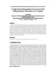
F i g . 2 Response of adaptive gain SMC during set point change for model A
H. J. THAM et al., Sliding Mode Control for a Continuous Bioreactor, Chem. Biochem. Eng. Q. 17 (4) 267–275 (2003)
271
The results for adaptive gain SMC is shown in figure 2. The responses for, both, the controlled output and input are smooth. However, a delay in evolution of substrate concentration is observed. This can be seen more clearly from the graph showing the evolution of the sliding function. It is clear that the controller is taking more than 0.5 h before driving the state back to the sliding surface, hence resulting in the delay. From the above results, it is obvious that the gains calculated are too small to force the state back to the sliding surface when a perturbation in the set point occurs. But once it reaches the sliding surface the control action is not over stressed as it can be seen from the plot of du/dt vs. time. Unlike in the fixed gain approach, the adaptive gain approach showed very little variation in du/dt with time. From these two studies it can be seen that high fixed gain approach should be used to drive the state quickly towards the sliding surface, soon after the perturbation in set point occurs. But once the state is near the sliding surface, adaptive gain approach should be used to minimise over stressing of control. We combined these features in the control law for the hybrid approach. Hybrid approach
To compare the performance of the hybrid approach with the fixed and adaptive gain approaches, the same set point changes to the system were made. If the sliding function was outside the range 0 ± 0.1, from the sliding surface, fixed gain was used. If the sliding function was with in the above range from the sliding surface, adaptive gain was used. The performance of the hybrid approach, which combined the fixed gain, and adaptive gain approaches, is shown in figure 3. Its performance is also compared with the PI controller. From the results, it can be observed that changes in both input and output displayed by the hybrid approach are smooth. The control response was immediate and after the set point was reached, the control action was minimal. The hybrid control exhibited the good features of both, fixed gain and adaptive gain controller. The PI controller also showed satisfactory response but there is a small abrupt change in the input signal. Nevertheless, both controllers show almost the same response time and no offset was observed in both cases. Since hybrid approach showed better control response, further simulations were done with this controller for various set point changes and disturbances and its performance compared with the PI controller.
F i g . 3 Performance of hybrid approach SMC for set point tracking as compared with PI controller
Set point change
Previous example depicts the changes in control input and output with respect to a small set point change. Figure 4 shows the response of the
F i g . 4 Responses of SMC during large set point change for model A.
272
H. J. THAM et al., Sliding Mode Control for a Continuous Bioreactor, Chem. Biochem. Eng. Q. 17 (4) 267–275 (2003)
controller when a large set point change was made to the system. The set point was changed from an initial substrate concentration of 0.523 g l-1 to 1 g l-1 at t = 0.5 h and later lowered to 0.5 g l-1 at t = 5 h. Again it can be seen that the regulation of substrate concentration is smooth with SMC. For PI controller, overshoots are observed in the output variable, and also the changes in the control input are much more than that of SMC. External disturbance rejection
Figure 5 presents the performance of the controllers in dealing with external or load disturbances. A step disturbance in the inlet substrate concentration (gsin) was introduced by decreasing it by 25 % from the nominal value (25 g l-1 to 15 g l-1) at t = 0.5 h. The disturbance is completely rejected by SMC by 2 h. For the PI controller, even after 5 h, the effect of disturbance was not completely rejected and offset is observed. It is clear that the disturbance affected the system under PI controller more than that under SMC. For SMC, after the first disturbance, the substrate concentration drops from 0.1 g l-1 to 0.08 g l-1 as compared with 0.071 g l-1 for the PI controller. This shows that SMC is faster in reacting to the perturbations as compared to the PI controller. At t = 5 h, the inlet substrate concentration was increased by 13 %, from 15 g l-1 to 17 g l-1. The response of the controllers is similar to the respective earlier responses to the disturbance.
F i g . 5 Disturbance rejection performance of SMC for change in gsin
Process parameter changes
To test the robustness of the controller, the process was subjected to about 50 % change in the nominal values of all quantities, i.e. mmax, Yx/s, Ki and Ks. The results are shown in figure 6. SMC once again proved robust, as it is able to bring the substrate concentration back to its steady state value in about 1 hour despite the large changes in all the parameter values. In case of PI controller, the performance is affected by these drastic changes in the parameter values and an offset is observed, as the controller is not able to regulate the substrate concentration back to the desired value. Invariance property
The closed loop response against different inlet substrate concentration with changes in set point was also studied for SMC and compared with the PI controller. Figure 7 shows the responses for two different inlet substrate concentration, i.e. gsin = 20 g l-1 and 10 g l-1. The initial value of substrate concentration is 0.528 g l-1 and the set point is 0.2 g l-1. For SMC, the closed loop responses for both inlet substrate concentrations are almost identical, i.e. exponentially regulated towards 0.2 g l-1. This can
F i g . 6 Process behaviour of SMC system for parameter changes
H. J. THAM et al., Sliding Mode Control for a Continuous Bioreactor, Chem. Biochem. Eng. Q. 17 (4) 267–275 (2003)
273
be considered to be an invariant behaviour against the difference in the value of gsin. For PI controller, the difference in the response for the two inlet conditions is quite obvious. For gsin = 10 g l-1, the response of the controller is smooth with the substrate concentration reaching the set point with a small undershoot. But for gsin = 20 g l-1, there is a large undershoot and a small offset is also observed before the set point is finally attained. For the dilution rate, it is clear that SMC reacts faster by reaching the corresponding equilibrium value than the PI controller. Results for model B
The improved SMC was also tested for the case B model. Based on the control output response, the controller design parameter c was chosen to be 5. As in the case A, the fixed switching gains were calculated using eq. (13), based on operating region and the range of parameters as given in table 2. The calculated fixed gains15 used in the simulation are Y1 = 7, Y2 = 1, Y3 = 6, Y4 = 7 . Figure 8 shows the dynamic responses of the controllers during set point changes. The set point was changed from 4.83 g l-1 to 4.0 g l-1 at 1 h and again changed to 5 g l-1 at 30 h. The evolution of the control output is smooth for both controllers. It is found that the system with PI controller has a shorter time response, though initially it shows some undershoot. For the second set point change, the same results as the first change are observed for both controllers. SMC takes a longer time in attaining the new set point and the PI controller shows a shorter time response with a small overshoot. For the control input, it is obvious that SMC requires larger control moves compared with the PI controller. SMC almost reaches saturation in the input signal for the first set point change, while the input of PI controller drops to 0.15 h-1 only. The second change shows the SMC with control input up to 0.5 h-1 compared to 0.25 h-1 for the PI controller. These results show that SMC requires larger control effort than PI controller to produce the desired response. Figure 9 illustrates the closed loop response of the system subjected to load changes. A 10 % increment in gsin was introduced at 1 h. Another load change was made at 30 h when gsin was decreased by 18 %. From the results, it is clear that for the system with SMC, the effect of the disturbances is very minimal on the control output. For the PI controller, the effect of disturbance is clearly seen with big changes observed in the control output. Offset is also observed for the PI controller. The change in dilution rate with time is not much different for both SMC and PI, but SMC responds quickly, resulting in faster rejection of the disturbance.
F i g . 7 System behaviour of SMC with different gsin during set point change
F i g . 8 Performance of SMC for set point tracking for model B
274
H. J. THAM et al., Sliding Mode Control for a Continuous Bioreactor, Chem. Biochem. Eng. Q. 17 (4) 267–275 (2003)
Figure 10 shows the response for both the controllers when mmax was changed from a value of 0.48 h-1 to 0.42 h-1 at 1 h, and later increased to 0.45 h-1. The result shows that the effects of the quantity variation are quickly corrected by SMC. PI controller is not able to bring the state back to the desired value for both changes. The trend of control input changes for both controllers are very similar to that of external disturbance rejection as shown in figure 9, i.e. SMC has a faster change compared with the PI controller. Figure 11 represents the closed loop response of the system for two different yields, Yx/s = 0.4 and Yx/s = 0.3. The system is regulated to a new set point of 3 g l-1 from its initial value of 4.8 g l-1. It is found that the closed loop responses of SMC for both cases are identical and almost overlap (line 1 & line 2) with one another. The dilution rate quickly reaches the saturation and remains there for a very short time so that the state can be rapidly brought to sliding surface. For the PI controller, the responses for the two 'Yx/s' values are different in their regulated paths towards the new set point (line 3 & 4). For Yx/s = 3.3, the substrate mass concentration drops below 3 g l-1 (i.e. undershoots) for a period of 10 hours before reaching the set point. From the above results, it is noted that for large set point changes, SMC works better compared with the PI controller. It is because the set point change is a perturbation to the transformed SMC system. PI controller produces satisfactory control response only for small step changes, which is more prominently observed from the simulation results for model B system. These results also show that SMC is not model dependent as the system behaviour is very similar for both case A and case B models.
F i g . 9 Performance of SMC during disturbance rejection for model B.
Conclusions This study has presented the application of SMC to two bioprocesses represented by different kinetic models. SMC using both deterministic approach and adaptive approach in determining the switching gains, were studied. An improved SMC, combining these two approaches, is applied for substrate concentration control using dilution rate as the control input. The excellent performance of the hybrid approach to SMC as compared with PI controller, especially in dealing with disturbance rejection and process parameter variation, is shown by simulation for two different fermentation models. SMC has also proven to be robust when tested with step change of more than 50 % in set point, external disturbance and parameter variation. The invariance feature of the SMC also indicates that uncertainties
F i g . 1 0 System behaviour of SMC during variation in mmax in model B
H. J. THAM et al., Sliding Mode Control for a Continuous Bioreactor, Chem. Biochem. Eng. Q. 17 (4) 267–275 (2003)
gx D e1 e2 Ki Ks t u Yx/s
– – – – – – – – –
Yp/x – a b
– –
m mmax s Y
– – – –
275
cell concentration, g l-1 dilution rate, h-1 error state, g l-1 error state as defined by equation (10), g h-1 l-1 inhibition constant, g l-1 saturation constant, g l-1 time, h control input yield coefficient for cells based on substrate consumed, g g-1 yield coefficient for product based on cells produced, g g-1 defined by equation 5, g-1 h-1 l non-growth associated specific production rate, h-1 specific growth rate, h-1 maximum specific growth rate, h-1 sliding function switching gain
References
F i g . 1 1 Process behaviour during set point change with variation in Yx/s model B
in loads and parameters would not affect how the closed loop system behaves, proving the robustness of SMC against uncertainties. SMC design is relatively simple and no tuning effort is required. It can be considered as a good alternative control system to be applied to nonlinear systems such as bioprocesses. However, the proposed approach to SMC requires online measurement of full state variables and prior knowledge of all the parameter values in the kinetic model. List of symbols
gp gpm gs gsin gs*
– product concentration, g l-1 – limiting product concentration, g l-1 – substrate concentration, g l-1 – inlet substrate concentration, g l-1 – set point for substrate concentration, g l-1
1. Slotine, J. J. E., Li W., Applied Nonlinear Control, Prentice Hall, N.J, 1991. 2. Shimizu, K., Adv. Biochem Bioeng, 50 (1993) 66. 3. Bastin, G., Dochain, D., On-line Estimation and Adaptive Control of Bioreactors, Elsevier, Amsterdam, 1990. 4. Sira-Ramirez, H., Int. J. Control 57 (5) (1993) 1039. 5. Emelyanov, S. V., Variable Structure Control Systems. Nauka, Moscow, 1967 (In Russian). 6. Itkis, U., Control Systems of Variable Structure, Wiley, N. Y., 1976. 7. Utkin, V. I., IEEE Trans. Automat. Contr. 22 (2) (1977) 212. 8. Hung, J. Y., Gao, W., Hung, J. C., IEEE Trans. Ind. Electron. 40 (1) (1993) 2. 9. Zlateva, P., Control Eng. Practice, 4 (7) (1996) 1023. 10. Zlateva, P., Bioprocess Engineering, 16 (1997) 383. 11. Zlateva, P., Proc. IEEE Workshop on VSS (1996) 61. 12. Shuler, M. L., Kargi, F., Bioprocess Engineering: Basic concepts, Prentice Hall International, New Jersey, 1992. 13. Fliess, M., IEEE Trans. Automat. Contr. 35 (9) (1990) 994. 14. Tham, H. J., Hussain, M. A., Ramachandran, K.B., Proc. RSCE (2000) Singapore. 15. Tham, H. J., Sliding Mode Control for Continuous Bioprocesses, Master's Thesis, University of Malaya, 2001. 16. Simutis, R., Oliveira, R., Manikowski, M., Feyo de Azevedo, S., Lubbert, A., J. Biotechnol. 59 (1997) 73. 17. Agrawal, P., Koshy, G., Ramseier, M., Biotechnol. Bioeng. 33 (1989) 115.