the core of a hardware software co-synthesis system. I Introduction. An embedded system is a special purpose computer con- sisting of one or more controllers ...
Software Scheduling in the Co-Synthesis of Reactive Real-Time Systems � Pai Chou, Gaetano Borriello Department of Computer Science and Engineering University of Washington, Seattle, WA 98195 Abstract { Existing software scheduling techniques limit the functions that can be implemented in software to those with a restricted class of timing constraints, in particular those with a coarse-grained, uniform, periodic behavior. In practice, however, many systems change their I/O behavior in response to the inputs from the environment. This paper considers one such class of systems, called reactive real-time systems, where timing requirements can include sequencing, rate, and response time constraints. We present a static, non-preemptive, ne-grained software scheduling algorithm to meet these constraints. This algorithm is suitable for control-dominated embedded systems with hard real-time constraints, and is part of the core of a hardware/software co-synthesis system. I Introduction
An embedded system is a special purpose computer consisting of one or more controllers and peripheral devices. A reactive system is an embedded system that changes its I/O behavior in response to inputs from the environment. This is in contrast to those systems with a uniform periodic behavior that is independent of their input. Many reactive systems must also meet hard timing constraints of various types imposed by the devices' protocols or by the required system behavior. These systems are referred to as reactive real-time systems. Esterel [1] and StateCharts [4] have been used for specifying reactive systems. Reactive behavior can be succinctly and conveniently captured with parallelism and watchdogs. A watchdog is a wait-on-signal statement that encloses a statement block, and breaks control ow out of the block upon receiving the signal. Both Esterel and StateCharts assume an idealized timing model,
� This work was supported by NSF under Grant MIP-8858782 and DARPA under contract N00014-J-91-4041.
where simple computations are assumed to take zero time to perform. However, lengthy computations that violate this assumption are extracted and treated as external signals, and timing constraints cannot be speci ed on them for scheduling. While this assumption simpli es semantics, it also restricts the class of applications that can be speci ed. The watchdog-concurrency reactive programming model has been augmented with timing constraints in [2]. The system behavior is divided into a number of modes. A mode speci es a scope within which a set of timing constraints must be met, until one of the watchdogs detects an event and disables, or causes a transition out of, the mode. When such a transition is initiated, each concurrent branch to be disabled is scheduled to run until a safe exit point is reached. This enables interleaving while maintaining the integrity of I/O protocols and program state. A timing constraint speci es a minimum or a maximum time separation between the start times of two operations. Elementary operations, such as reading and writing an I/O port or computations, take some bounded amount of time to execute and are not preemptable. Other operations, speci cally polling loops that wait for an input value, can iterate inde nitely, and are said to have unbounded delays. When there are multiple paths between two operations, the maximumtiming constraints are de ned for those paths with only bounded-delay operations. We classify the constraints into sequencing, rate, and response time. A sequencing constraint speci es the separation between the start times of two operations in the same mode and same iteration without intervening unbounded delay operations. Sequencing constraints are commonly found in I/O protocols of peripheral devices. These protocols consist of a sequence of read and write steps. A rate constraint speci es the separation between the start times of two consecutive iterations of a loop. Note that the rate constraint holds only between successive iterations until the loop exits. A loop with a rate constraint can have a body with sequencing constraints. A
w in G with edge e between them, �(w) , �(v) � e . In the extended scheduling problem, we must also consider the safe exit points, disables, and the intermodal constraints. A set of safe-exit points S include all leaves in G and any speci ed internal safe exit points. The set of disable nodes D is a subset of S . A legal exit point is a safe exit point whose peer branches in G are at their safe exit points. Formally, let P (c) be the set of vertices scheduled before c (that is, fv : �(v) < �(c)g). A safe exit point c is legal if every v 2 P (c) is safe with respect to c and �. A vertex v is safe with respect to c and � if v 2 P (c) and either (i) v is a safe exit point, or (ii) all children of v in G are safe with respect to c and �. Intermodal constraint edges are similar to their intramodal counterparts. An intermodal edge (v ; w ) with a nonnegative weight e x y associated with the x ! y transition requires that w be scheduled no earlier than e x y time units after v 's scheduled start time. An intermodal edge (w ; v ) with a negative weight e y x II Scheduling Problem Formulation associated with the x ! y transition requires that w be scheduled no later than ,e y x time units after v 's The input to this problem is a constraint graph. It scheduled start time. is an extended version of the constraint graph used in relative scheduling [6]. The vertices represent operations III Scheduling Algorithm and the edges represent timing dependencies. Each graph is required to have a single entry point, or anchor. Each vertex v has an non-negative integer execution delay � (v), A Intramodal Scheduling shown in Fig. 2 as a value after the `/' in the node. In Although intramodal scheduling can be solved using the basic problem, each graph corresponds to a mode and serialization [5] and start time assignment [6], we present contains only bounded delay operations. Timing constraints are represented by a set of directed here a combined algorithm, that is adaptable to interedges. All edges have integer weights and are catego- modal scheduling (Section B) and can be easily modi ed rized as either forward edges (those with zero or positive to use di�erent heuristics. The input is an intramodal weights) or backward edges (those with negative weights). constraint graph, and the output is a schedule for the A forward edge from vertex v to vertex w with weight start times. The algorithm is shown in Fig. 1. The algorithm is called with three parameters. The e indicates that the start time of w must be scheduled at least e time units after v's scheduled start time. rst parameter G is a modal constraint graph. The secA backward edge from vertex w to vertex v with weight ond parameter is the anchor a of the graph. Every vertex e indicates that the start time of w must be scheduled must be reachable from a in G along non-negative weight no more than ,e time units after v's scheduled start edges, as explained in section II. The third parameter c time. We call the constraint graph limited to forward is the current vertex being traversed. It is initially set to edges only the forward constraint graph and label it G . a, and it separates the subgraph already serialized from In all modes, all nodes are required to be reachable from the rest of the graph. This algorithm performs a variation of topological the anchor, or start node, along a path in G . The basic problem is de ned as follows. Given a con- traversal, starting from a. A vertex is a candidate to be straint graph G and an anchor vertex a, derive a valid serialized next if all of its predecessors in G have been serial schedule. A schedule is a mapping of the vertices to serialized. If a vertex v is chosen from the candidate set integers representing their start times relative to the an- to be visited after c, then a forward edge is added from chor a. Serialization requires that operations be assigned v to all other successor candidates u of c. When adding nonoverlapping times. That is, if vertex v has duration a forward edge (v; u), we assign the edge weight e = � (v) and is assigned start time �(v) then no other event Max(� (v); L (u) , L (v)), where L is the longest path is assigned a start time between �(v) and �(v) + � (v). length from the anchor a to the vertex, as computed by A schedule is valid if it satis es all the constraints. In- the BellmanFord longest paths algorithm. The justi tramodal constraints are satis ed if for all vertices v and cation for the edge weight is that since u is to be ordered maximum rate constraint is well posed only if the loop does not contain operations with unbounded delays. A response time constraint is a constraint on a mode transition. The path is de ned to be from the last iteration of the rst mode to the rst iteration of the next mode. Response time constraints are also referred to as intermodal constraints. Sequencing constraints are also called intramodal constraints. For the purpose of scheduling, a rate constraint can be formulated as an intramodal constraint. This paper presents a static scheduling algorithm for producing a sequential program to meet both intramodal and intermodal timing constraints. Static scheduling is necessary because dynamic scheduling cannot guarantee that constraints will always be satis ed [7]. In the next sections, we formulate the scheduling problem in terms of a graph model and then present the scheduling algorithm.
v;w
v;w
f
f
f
x
v
v
y
;w y
x
;w
y
x
w ;v
y
w
x
;v
v;w
v;w
w;v
w;v
f
f
f
vu
a
a
a
Serialize(Graph G; anchor a; candidate c) f La := Single source longest paths(G, a); if positive cycle found, return Fail ; C := topological successors of candidate c; if (C is empty ) return schedule with �(v) = longest path from a; D := C ; while (D not empty) f v := SelectSuccessor(D); B: foreach u 2 C , fvg f add edge (v; u) to G, with weight evu = Max(�(v); La (u) , La (v)); /* delay all successors by at least �(v) */
g
Serialize(G; a; v); found) return schedule; /* else - positive cycle or backtrack */ Undo step B; g /* while */ return Fail; /* no more candidates */ if (schedule
g
k
a/2
K A 7 2 ? A
k A-4 c/1
�k, 1,�s/1?k 2@1 u/2 � @RAAt/1k 2 �3 ?k�� v/3
after v, u cannot start until after v completes, or after a longer minimum constraint from the anchor. Note that the edge (v; u) could already exist, but it can only be a backward (negative weight) edge representing a maximum constraint from u to v. Since we order v before u, this maximum constraint is always satis ed, and therefore no information is lost by converting (v; u) into a forward edge. A positive cycle in the constraint graph implies an infeasible constraint, since it requires a node to be scheduled later than its own start time. If the addition of new edges results in positive cycles, then the algorithm backtracks. The next candidate is considered, until a schedule is found or all candidates have been exhausted. Fig. 2 illustrates the algorithm. This algorithm is guaranteed to nd a feasible ordering if one exists. At any level in the recursion, the algorithm cannot fail unless all possible orderings of the remaining unserialized nodes are infeasible. Since there is a feasible order, this will not happen. The correctness of the algorithm can be proved by induction, and is sketched as follows. Assuming a valid ordering exists, the basis is that the anchor a is correctly ordered. Inductive hypothesis is that everything from the anchor up to the current vertex c is in the correct order. Suppose v is the next vertex in a valid ordering, then L (v) is exact as the longest forward path from a to v. A forward edge (v; u) is added for each peer u of v. The edge weight � (v) is a necessary minimum constraint by de nition of serialization, because no a
k
v/3
Vertices a, c have been serial- (b) Suppose we pick u to serialize ized. The successor candidates of c next. We add an edge from u to its are fu;s; tg but not v since v is a peers s and t, with the edge weight successor of u. of �(u) = 2 in both cases. However, this results in a positive cycle (a; u;t). (a)
k
k ?k
a/2
� 2 AKA -4 7� ? ��� c/1k@@R1AA kL�a=(u7) ,, L3 a=(t4)t/1k u/2 2 2 ?k ? s/1 k v/3
Suppose t is selected after c. We add edges (t; s) and (t; u), with edge weights 1 and 4, respectively. No positive cycle is formed. The successor candidates of t are fu; sg. (c)
Fig. 1: Intramodal Scheduling Algorithm
k
a/2
�2 AK 7 � ?A -4 A ���1,2c/1k 1 kX, �-(Xu) s/1k?@@A@RAA u/2 2 ? �(uX) =X2 XXz t/1k
a/2 2 A K c/1 A -4 A 1A 4 t/1 �(u)
kP�P @@R k ?k PPPq k
u/2 2
s/1
v/3
Suppose u is chosen to be serialized after t. We add the edge (u;s) and no positive cycle is formed. The successor candidates of u are fv; sg. The graph can be completely serialized in one more step (not shown). (d)
Fig. 2: Example of Intramodal Serialization computations can overlap. If L (u) , L (v) > � (v) then it is also a necessary constraint. The weight is exact if u is to be ordered immediately after v. Since the algorithm backtracks to try all possible vertices, it nds a solution if one exists. Note, however, that in the worst case, an exponential number of orderings may be attempted. The complexity of this scheduling problem is NP-hard. There exists a simple transformation to this problem from the \Sequencing with Release Times and Deadlines" problem, which is NP-complete in the strong sense [3]. It is possible to substitute the SelectSuccessor() function (just above label B) with a heuristic function that selects vertices in a better order and considers the e�ects of choices on scheduling disables and safe exit points. To select a good candidate to serialize next, we use a \slack" function as a heuristic. Slack is a measure of how urgently a vertex should be serialized. Smaller slack implies higher priority. A heuristic for choosing operations on a path with a disable is to schedule the disable near the safe exit points such that the amount of code remaining before reaching the safe exit points is minimized. This code will need to be executed at the exit to the mode and impacts not only code size but more importantly, the ability to meet response time constraints. a
a
� - 6 Mode A ? k a/1 X 6 � � 6 3Xzc/2k �9k b/2 , 63 -8@ @@R k, ,2 -10 3 d/1X � � 9 � 3 kX3Xz �-44X�z�:f/2k e/1 k 6 Mode B g/2 ? � ?-
�� kXXz k 9k � XXz k� 9�� 6 �� XXz k 9k � : XXz k��� 6 ? k � � XXz k 9k �
b/2
-8
e/1
b/2
6 3 3 3
6
a/1
d/1
g/2 3 a/1
3 c/2 2
4 f/2 -4 -10
3 c/2
An intermodal constraint graph. (b) Construct a graph with copies The response time edges associated of mode A before and after mode B. with the A to B transition are Serialization starts on the anchor of f(b; d); (c; d); (e; b)g; those for the B, which is the vertex d. B to A transition are f(g;a); (c; f )g. (a)
k d/1 � � � 9 k3 �91�2�-���:f/2k e/1 k -4 6 g/2 3 ? -10 kX3Xz a/1 3 � k k c/2 b/2 X 3X z k 6 -8�� d/1 9 � 3 k �91�2�-���:f/2k e/1 -4
k 3 d/1 � � � 9 k �91�2�-���:f/2k e/1 k -4 6 g/2 3 ? -10 �6 a/1kX3Xz k � 9 � k c/2 b/2 2� X 3X � 9 � z k 6 -8 � d/1 �3 1 - f/2k 9 � k e/1 �9�2�-4���: k
k
g/2
Another graph is constructed, where the predecessor and successor of A are both the serialized version of B. The anchor for this serialization is a. (c)
g/2
After a complete ordering is obtained for mode A, and since mode B is also totally serialized, the intermodal constraints are sufficient for both serialized graphs. The final orderings are (a; c; b) and (d; e;f; g). (d)
Fig. 3: Example of Intermodal Serialization B Intermodal Scheduling
Intermodal scheduling, the scheduling of modes to meet intermodal constraints, can be viewed as an extension to the intramodal version. Instead of scheduling each mode in isolation, now we must also consider intermodal constraints. Fig. 3 shows an example of our method of intermodal serialization. Since modes A and B alternate we serialize B by generating a graph consisting of two copies of A, and one of B , with one A before the B and one after. Additional precedence edges are added from all legal exit points of a preceding mode to the anchor of its successor to ensure that all of a mode's nodes are executed before control is passed to the next mode. After B is serialized, we repeat the process for A with two copies of the serialized version of B , one before and one after A. Should no feasible solution be found for serializing A, the algorithm backtracks to nd a new feasible solution for B before retrying A. In addition, intermodal constraints can be relaxed by considering di�erent legal exit points as more schedules for the various modes are completed.
IV Conclusion
Software synthesis is an emerging eld in the automation of embedded system design. We speci cally target the co-synthesis of embedded reactive real-time controllers, where the software is characterized by real-time constraints on control-dominated programs. Our focus is on low-cost systems that exploit microcontrollers or core processors and do not use an operating system to implement dynamic scheduling. In this paper, we have presented an algorithm for software scheduling based on an extended model of timing constraint speci cations as described in [2]. It is more general than earlier work in this area. The concept of safe exit points allows us to consider the e�ects of watchdogstyle constraints used to describe reactive behavior. A new scheduling technique is guaranteed to nd a static schedule that meets all the sequencing, rate, and response time constraints. The speci cation methods and scheduling algorithm are part of the Chinook hardware/software co-synthesis system currently under development at the University of Washington. References
[1] F. Boussinot and R. De Simone. The Esterel language. Proceedings of the IEEE, 79(9), Sept. 1991. [2] P. Chou, E. Walkup, and G. Borriello. Scheduling issues in the co-synthesis of reactive real-time systems. Technical report, Univ. of Washington, Dept. of Computer Science, Mar. 1994. [3] M. R. Garey and D. S. Johnson. Computers and Intractability: a Guide to the Theory of NPCompleteness. W. H. Freeman and Company, 1979.
[4] D. Harel. StateCharts: a visual formalism for complex systems. Science of Programming, 8, 1987. [5] D. C. Ku and G. De Micheli. Constrained con ict resolution and resource sharing in Hebe. Integration { The VLSI Journal, 12:131{165, Dec. 1991. [6] D. C. Ku and G. De Micheli. Relative scheduling under timing constraints: algorithms for high-level synthesis of digital circuits. IEEE Transactions on Computer-Aided Design, 11(6), June 1992. [7] J. Xu and D. L. Parnas. On satisfying timing constraints in hard-real-time systems. IEEE Transactions on Software Engineering, 19(1):70{84, Jan. 1993.