CALL, which is a profiling tool for interacting with the code in an easy, simple and direct way. New features .... of calls of any MPI function or the overlap between commu- nication and .... ios for the same code âfrom few large messages to many.
Software Tools for Performance Modeling of Parallel Programs Diego R. Mart´ınez1 , Vicente Blanco2 , Marcos Boull´on 1 , Jos´e C. Cabaleiro1 , Casiano Rodr´ıguez2 , and Francisco F. Rivera1 1
University of Santiago de Compostela Dept. of Electronics and Computer Science Santiago de Compostela, A Coru˜na. SPAIN {diegorm,marcos,caba,fran}@dec.usc.es Abstract This paper presents a framework based on a user driven methodology to obtain analytical models of MPI applications on parallel systems in a systematic and easy to use way. This methodology consists of two stages. In the first one, instrumentation of the source code is performed using CALL, which is a profiling tool for interacting with the code in an easy, simple and direct way. New features are added to CALL to obtain different performace metrics and store the performance information in XML files. Using this information, an analytical model of the performance behavior is obtained in the second stage by means of R, a language and environment for statistical analysis. The structure of the whole framework is detailed in this paper, and some selected examples are used to show its practical use.
1
Introduction
We can classify the different approaches to performance modeling as the combination of three categories: analytical modeling, simulation modeling and measurement [14, 23]. Analytical models are fast and efficient since the behavior is described through mathematical equations. They have been less successful in practice for predicting detailed quantitative information about program performance. It seems that simplicity and accuracy are contradictory goals. Memory hierarchies, asynchronous events and embedded processor parallelism make it difficult to harmonize them. On high performance computers which exploit multiprocessor parallelism this problem gets even worse, as the performance of the network and the actual communication patterns often have a non negligible unpredictable effect [23]. In fact, c 1-4244-0910-1/07/$20.00 �2007 IEEE.
2
La Laguna University Dept. Statistics and Computer Science La Laguna, Tenerife. SPAIN {vblanco,casiano}@ull.es
the two currently most used parallel performance analytical models, BSP [21] and LogP [7] are distributed memory oriented and simplify the parallel architecture to four or five parameters. Sometimes instead of a set of analytical formulas the model provides an algorithm. For example, Vikram S. Adve and Mary Vernon presented in [1] an algorithmic model that is the high-level component of a two level hierarchical model for shared memory machines. The higher level component represents the task level behavior of the program (task scheduling, execution and termination and process synchronization). Assuming the existence of a lower level model component providing the task execution times, the higher level produces the overall execution time. Simulation modeling constructs a reproduction not only of the time behavior of the modeled system but also its structure and organization. It plays an important role in architecture design. Simulation modeling can be more accurate than analytical modeling but is more expensive and time consuming and can be unaffordable for large systems. Empirical experimentation is an irreplaceable task in any science. Measurement methods allow us to identify bottlenecks on a real parallel system performance. This approach is often expensive because it requires special purpose hardware and software. Performance measurement can be highly accurate when a correct instrumentation design is carried out for a target machine. As in any science field, real systems are not always available. Some approaches [6, 8, 19] combine empirical experimentation, analytical modeling and perhaps some lightweight form of simulation. The experimentation and simulation is used to characterize the application while the analytical model is used to predict the performance behavior in terms of the characterization of the algorithm and the knowledge of the platform. The work in [6] is representative of a set of strategies consisting of measuring and (analytically) modeling the sources of overhead in the parallel program. The sources of overhead are partitioned into mu-
tually exclusive categories that have to be significant to allow the programmer to interpret the results in terms of the program. A further level of abstraction is provided by [8], where the performance categories can be described using a performance specification language. The work of Snavely et al. [19] also combines empirical experimentation, analytical modeling and simulation. As systems become more complex, as is the case of multiprocessing environments or distributed systems, accurate performance estimation becomes a more complex process due to the increased number of factors that affect the execution of an application. As well as relatively static information, such as CPU speed, memory size or network capacity, there are other dynamic parameters, such as CPU or network loads, that must be taken into account in the performance estimation. Moreover, most of these dynamic parameters may not be known until run time [12]. Therefore, some performance estimations must be performed at launch time, when the resources on which the program has to be run are known, and some others must be done at run time, because assumptions made by the performance estimator must be reconsidered if they are significantly wrong [9]. This paper describes a framework based on a two stages methodology to obtain analytical models of MPI applications on parallel systems. Section 2 introduces a short state of the art in analytical models for performance analysis. The methodology to obtain analytical performance models is described in section 3. This methodology is based on an enhanced version of the CALL instrumentation tool [3, 5] and on the R statistical package [18]. Section 4 shows a case study of the proposed methodology. Finally, Section 5 presents the main conclusions of this work.
2
Analytical Models for Performance Analysis
Performance models can be grouped into three categories: analytical modeling, simulation modeling and measurement [14, 23]. Each category of models can require significant work to develop. Although analytical approaches are generally less accurate than simulation approaches, they have the advantage that it is relatively less time consuming than the simulation approach. Analytical models, based on a concise characterization of the program, are more amenable to a high level interpretation of the parameters in the model and to a characterization of the sensitivity of architectural elements. Besides, parametric models which allow the study of performance scenarios through extrapolation can be produced by analytical approaches. In addition, analytical model information can be useful in load balancing strategies [13]. Prophesy, DIMEMAS and PACE are examples of perfor-
mance tools that use analytical models. The Prophesy [20] infrastructure automates the performance analysis and modeling processes. It includes automated instrumentation, extensive databases for archiving the performance data, and an automated analytical performance model builder for parallel and distributed applications. DIMEMAS [2] is an eventdriven simulator that predicts the behavior of MPI applications. The execution behavior on the target architecture is obtained from a tracefile and a configuration file that models the architecture. The tracefile captures the CPU burst versus the communication pattern information of an execution of the application on a source machine. PACE [16, 11] is a performance prediction system that provides quantitative data concerning the performance of application running on parallel and distributed computing systems. The system characterizes the application and the underlying hardware on which the application is to be run, and combines the resulting models to derive predictive execution data. The proposed modeling framework helps the analyst in the process of tuning parallel applications and automatically performs some tedious processes, but it is not intended to substitute the analyst tasks. Its modular design makes it possible to introduce new tools in the framework, or even substitute current functionalities, with a minimal impact on the rest of the framework. Analytical models are obtained by a statistical analysis of measurements from real parallel executions. Therefore, the behavior of an application can be characterized in terms of parameters such as the problem size, the number of process or the effective network capacity.
3 The Modeling Framework A methodology to obtain analytical performance models of MPI applications is introduced in this section. Figure 1 shows a scheme of this methodology that consists of two connected stages. The whole process is almost transparent to the user because of the automatic connection between both stages. The first one implements the instrumentation of the source code so that information about the performance in each execution of the application is gathered and stored. In the second stage, an analytical model is calculated by means of a statistical analysis of the performance data obtained from multiple executions of instrumented code. This methodology is based on two tools: CALL and R. CALL [3, 5] is a profiling tool to interact with the code in an easy, simple and direct way. It controls external monitoring tools through CALL drivers that implement an application performance interface to those external tools. Therefore, CALL is a modular tool and new drivers are developed as new monitoring tools are taken into account. This feature also avoids the dependence of any specific monitoring tool. R [18] is a language and an environment for statisti-
Figure 1. Methodology scheme. cal computing and graphics. In our case, it is used to build analytical models from monitoring data. Some of the advantages of R are the capability to produce well–designed publication–quality plots easily, and the large number of R functions for effective data handling and data analysis. Besides, it is also highly extensible through the use of standard packages and user programs stored in script files.
3.1
The Instrumentation Stage
The instrumentation of the source code is implemented using CALL [5]. The user, using pragmas, sets CALL experiments which specify where to take observations about how the code is performing during its execution and the events to be observed. Therefore, specific kernels or functions that are relevant for the performance of the application may be modeled instead of the whole application. The information of the monitored parameters during the execution of the instrumented code is gathered and stored in XML files which verify a specifically designed Document Type Definition (DTD). The nature of monitored parameters is quite different as they can come from different sources such as timers, specific microprocessor counters or external monitoring tools. The access to this information is performed by CALL drivers. In figure 1 some drivers are shown as the NWS, Ganglia, MPI, PAPI and Paraver drivers. These drivers can be used together in order to simultaneously obtain performance measurements from different sources. The MPI driver monitors the number of processes, their
process identifier and the elapsed time of CALL experiments in MPI applications. The PAPI driver obtains information by means of PAPI [4]. PAPI specifies a standard application programming interface for accessing hardware performance counters available on most modern microprocessors. Some events, such as cache misses, float point instructions or conditional branch instructions among many others can be monitored in a CALL experiment using this driver. The NWS and Ganglia drivers are intended to be used in Grid environments where these tools are integrated in the middleware infrastructure for monitoring purposes. Network Weather Service (NWS) [22] is a distributed tool that monitors and dynamically forecasts the performance of network and computational resources. Ganglia [10] is a scalable distributed monitoring tool for high-performance computing systems such as clusters and Grids. All monitored parameters by NWS or Ganglia can be obtained through these CALL drivers. In the experiments, shown in section 4, the latency and bandwidth of the network were monitored using the NWS driver. Other parameters, such as CPU or memory utilization, can be accessed by the Ganglia driver. Paraver [17] is a flexible performance visualization and analysis tool that can be used to analyze parallel applications, hardware counters profile, operating system activity and many other issues. In a preinstrumentation stage, this tool can help to identify what parts of the source code are candidates for being monitored. Paraver traces of a CALL experiment can be obtained by the Paraver driver. These traces provide performance information, such as the number
Figure 2. R modules for the performance data manipulation. of calls of any MPI function or the overlap between communication and computation, that can be useful in the analysis stage. The call tree of user functions can be obtained by the definition of user events so that the information of the trace can be classified in terms of these user functions.
3.2
The Analysis Stage
The analysis stage is based on R [18]. The final aim of this stage is to obtain an analytical expression for the elapsed time of a CALL experiment parameterized by monitored parameters and some features of the code. Instrumentation data obtained from multiple executions of the instrumented code are loaded in the R environment, and then suitable data structures for the statistical analysis are automatically generated. Some data process, such as the combination of several monitored data to obtain derived parameters, can be performed at this point. Using these data structures, the analytical model is built by specifically designed R functions. The experimental data are fitted to an equation that describes the model in terms of the monitored or derived parameters. The user can supply this equation, but if there is not any knowledge about the behavior of the performance of the application, the best approach from a generic set of equations is selected to be used as the first solution of an iterative tuning process. Several R modules were developed to help the performance analyst in the process of managing the huge amount of performace information gathered during the instrumentation state. These R modules are organized to allow the user to obtain in a few steps graphical information about
the proposed analytical model. In figure 2 we show how the R modules are organized. It consists of three main modules: IMPORT, FIT and DRAW. The IMPORT module transforms the XML data from the instrumentation stage into R structures. The analytical model is obtained by means of FIT. In order to obtain a fine analysis, the user can incorporate relevant information into this module like a preliminary guess formula. Information is extracted from the data (selectData) and the outliers are detected (outliers). Then the model is performed by an iterative process from the preliminary formula (fit) and relevant information of the model is print out (print). Finally, the DRAW module automatically builds appropriate figures using the information from the model. The user can redefine the default views of these figures like the title or the axis labels.
4 Case Study: Matrix Product To show the practical use of this framework, three different versions of the parallel matrix product of two N×N matrix of single-precision floating-point numbers have been used. The matrix product was chosen because very different implementations can easily be considered, and the obtained models can be contrasted with the expected behavior. Figure 3 shows the pseudocode of these codes. The distribution of both A and B matrices (MPI_Scatter and MPI_Bcast) and the number of computations are the same in all cases. The differences are in the number and size of the messages in the collection of partial results (MPI_Gather). Case-1 performs one communica-
MPI Scatter(A) MPI Bcast(B) for i in 1:(N/P) { for j in 1:N { C(i,j)=0 for k in 1:N { C(i,j)+=A(i,k)*B(k,j) } } } MPI Gather(C) MPI Barrier
(a) CASE 1
MPI Scatter(A) MPI Bcast(B) for i in 1:(N/P) { for j in 1:N { C(i,j)=0 for k in 1:N { C(i,j)+=A(i,k)*B(k,j) } MPI Gather(C(i,*)) MPI Barrier } }
(b) CASE 2 MPI Scatter(A) MPI Bcast(B) for i in 1:(N/P) { for j in 1:N { C(i,j)=0 for k in 1:N { C(i,j)+=A(i,k)*B(k,j) MPI Gather(C(i,j)) MPI Barrier } } }
(c) CASE 3
Figure 3. Pseudocode of the three versions of parallel matrix product (C=A×B), where all matrix size is N×N and P is the number of process.
tion once the partial result is calculated in each process. In Case-2 there is one global communication for each row of the resulting matrix. There is one global communication for each element of partial result in Case-3. In order to minimize the effects of the overlap between communication and computation, a MPI_Barrier is executed after each MPI_Gather call. Therefore, three different scenarios for the same code –from few large messages to many small massages, with the same number of FLOPs– are taken into account. The goal of the experiment is to characterize the difference of the model if the number and size of communications increase. Therefore, the state of the network in the
execution of the programs has to be taken into account, specially in Case-2 and Case-3. The NWS driver of CALL was used to monitor the network parameters during the execution of the programs and, simultaneously, the elapsed time of CALL experiments and the number of cache L2 misses were measured through the PAPI driver. Different matrix sizes (100×100, 150×150 and 200×200) have been used.
4.1
Network Monitoring Using NWS
NWS manages a distributed set of performance sensors (network monitors, CPU monitors, etc.) from which it gathers readings of the instantaneous conditions. For example, effective latency and bandwidth between nodes of the network where a MPI application is running can be monitored. The effective latency is defined as the amount of time required to transmit a small TCP message to a target sensor and the effective bandwidth as the real speed at which a TCP message is sent. Both parameters are variable as the load of network may change during the execution of the application, specially on a Grid system. Often, the load of the network where a MPI application is running may be influenced by other processes that share the same network. Therefore, the effective latency and bandwidth of a network must be taken into account when the performance of parallel applications is analyzed. The NWS driver provides an easy way to use the NWS monitoring system. It is assumed that an independent NWS system is able to monitor the network where the instrumented code will be executed. In order to monitor the effective latency and bandwidth during the execution of the instrumentation code, the NWS driver reads a configuration file and a NWS activity is started at the beginning of the CALL experiment. The NWS activity monitors both the latency and the bandwidth during a CALL experiment. At the end of the CALL experiment, the NWS activity is stopped and the monitored values are gathered from the NWS memory server and stored in an appropriate XML file. In the analysis stage, the NWS data must be loaded in the R environment in a special way because there is no connection between each execution of a MPI CALL experiment and the monitored values of the NWS CALL experiment. A process to connect the monitored network variables and the rest of the variables is necessary. The information stored in CALL output files is essential in this process because some characteristics, such as the name of the nodes and the initial timestamp, are stored in CALL output files as attributes. In our experiments, monitored values of both effective bandwidth and latency were used to calculate the bandwith mean and the latency mean, respectively, for each execution of the program. Therefore, these two values were used as model parameters.
4.2
Results
The programs were executed several times in a cluster of six 3 GHz Intel Xeon biprocessors with a Gigabit Ethernet. Several noise programs were used to obtain different network behaviors. In particular, a continuous broadcast of a vector among the processors was used. The traffic of the network changes in accordance with the length of this vector. The following equation has been used as a first approximation in the analysis stage: t = A + B · MAC + C · L2CM ¯ + E · �log2 P� SC (1) +D · �log2 P� · NC · L ¯ B where t is the estimated time, MAC is the number of multiply-and-accumulate operations, L2CM the number of L2 cache misses and P the number of processors. The la¯ tency mean and the bandwidth mean are represented by L ¯ and B, respectively. NC is the number of global communications, and SC is the size of these communications. In the three cases, all the communications are collective so a logarithm factor must be included in the terms related to network parameters [15]. The coefficients (A, B, C, D and E) are obtained by R fitting the experimental values to this equation. An iterative process was used to obtain the appropriate model for each case. Negative coefficients were eliminated because they are incoherent with the physical meaning of the terms of equation (1). Besides, in this case study, coefficients with a standard error greater than 10% were also eliminated. The representation of the obtained models is shown in Figure 4. The figures on the left show the experimental values (◦) and the model output (×) in each case. The lines only represent the trend of the model for each matrix size. On the right hand, the distribution of the residuals of each model is represented. These graphics provide an estimation of the accuracy of the models. The obtained model for each case is the following: CASE 1: t(µs) = 280 + 0.0196 CASE 2:
N3 + 1.82 · L2CM P
(2)
N3 + 0.66 · L2CM P N (3) +4.9�log2 P� ¯ B
¯ is the mean bandwidth in Mbps, L ¯ the mean lawhere B tency in µs, and N the number of rows of the matrix. In the first case, the number of communications is small and the execution time depends almost exclusively on the number of computations. This fact agrees with the obtained model where the terms related to network parameters do not appear. The models of cases 2 and 3 include these parameters because of the increase of the number of communications. In these cases, the communication time has greater importance in total time than in case 1. In the last case, the latency has a special prominence because there is a huge number of communications but the length of the messages is small. Besides, in this last case, the high number of communications is responsible for the increase in execution time, so that the term related to cache misses is overshadowed. The coefficients of determination (R2 ) in each case are shown in table 1. The coefficient of Case-3 is low because in this case the number of communications is so large that there are other factors than those characterized by equation (1), such as network conflicts.
5 Conclusions A framework based on a methodology to obtain analytical models of MPI applications on multiprocessor environments is presented in this paper. The framework consists of an instrumentation stage followed by an analysis stage, which are based on the CALL instrumentation tool and in the R language, respectively. New drivers for the CALL instrumentation tool are written to obtain performance data from NWS and Ganglia systems. The CALL gathering performance data facilities were completely redesigned to obtain the data in XML format. This feature permits easy data manipulation on the analysis stage. Some R packages were developed to help the performace analyst to research in his analytical model, including the fast generation of graphical performace data for the proposed model as well as statistical information about the fitting process. As a case study, we present the analysis of the well know matrix product problem. We show the easy and fast results obtained using this tools practically without modifying the
t(µs) = 5000 + 0.0162
CASE 3:
N3 t(µs) = 360000 + 0.42 P N2 ¯ L +0.42�log2 P� P
Table 1. Coefficients of determination (R2 ). Case R2 1 2 3
(4)
0.9707 0.9525 0.7721
CASE 1 − Residuals
40 20
0
−20
0
60000
RESIDUALS (%)
100000
experimental model N=100 N=150 N=200
20000
time (usec)
60
CASE 1 − Model
4
5
2
4
5
CASE 2 − Model
CASE 2 − Residuals 40
6
−20
6e+04
RESIDUALS (%)
1e+05
experimental model N=100 N=150 N=200
4
5
6
2
3
4
5
# CPUs
# CPUS
CASE 3 − Model
CASE 3 − Residuals
20 0
0e+00
−40
2e+06
4e+06
RESIDUALS (%)
40
60
experimental model N=100 N=150 N=200
6
−20
3
6e+06
2
time(usec)
3
# CPUS
2e+04
time (usec)
6
# CPUs
20
3
0
2
2
3
4 # CPUs
5
6
2
3
4 # CPUS
Figure 4. Experimental measures and the model.
5
6
source code (we only introduce a few pragmas for the instrumentation). We also show detailed graphical and statistical information about the fittings for the analytical models proposed.
6
Acknowledges
This work was supported by the Spanish Ministry of Education and Science through TIN2004-07797-C02 and TIN2005-09037-C02-01 projects and through the FPI programme.
References [1] V. S. Adve and M. K. Vernon. Parallel program performance prediction using deterministic task graph analysis. ACM Transactions on Computer Systems, 22(1):94–136, 2004. [2] R. M. Badia, J. Labarta, J. Gim´enez, and F. Escale. Dimemas: Predicting mpi applications behavior in grid environments. In Workshop on Grid Applications and Programming Tools (GGF8), Seattle, WA, USA, June 2003. [3] V. Blanco, J. Gonzlez, C. Len, C. Rodrguez, G. Rodrguez, and M. Printista. Predicting the performance of parallel programs. Parallel Computing, 30(3):337–356, Mar. 2004. [4] S. Browne, J. Dongarra, N. Garner, G. Ho, and P. Mucci. A portable programming interface for performance evaluation on modern processors. The International Journal of High Performance Computing Applications, 14:189–204, 2000. [5] Call: A complexity analysis tool. http://nereida.deioc.ull.es/ call. [6] M. E. Crovella and T. J. LeBlanc. Parallel performance prediction using lost cycles analysis. In Proceedings of the 1994 ACM/IEEE conference on Supercomputing, pages 600–609, Washington, D.C., 1994. ACM Press. [7] D. Culler, R. Karp, D. Patterson, A. Sahay, K. Schauser, E. Santos, R. Subramonian, and T. von Eicken. LogP: Towards a realistic model of parallel computation. In 4th ACM SIGPLAN Symposium on Principles and Practice of Parallel Programming, May 1993. [8] T. Fahringer, M. Gerndt, G. D. Riley, and J. L. Tr¨aff. Specification of performance problems in mpi programs with asl. In 2000 International Conference on Parallel Processing (ICPP’00), pages 51–, Toronto, Canada, Aug. 2000. IEEE Computer Society Press. [9] I. Foster and C. Kesselman. The Grid2: Blueprint for a New Computing Infrastructure. Elsevier, Inc., 2004. [10] Ganglia monitoring system. http://www.ganglia.info. [11] S. Jarvis, D. Spooner, H. L. C. Keung, J. Cao, S. Saini, and G. Nudd. Performance prediction and its use in parallel and distributed computing systems. Future Generation Computer Systems special issue on System Performance Analysis and Evaluation, 2004. [12] N. H. Kapadia, J. A. B. Fortes, and C. E. Brodley. Predictive application-performance modeling in a computational grid environment. In 8th IEEE International Symposium on High Performance Distributed Computing (HPDC ’99), Los Angeles, Aug. 1999.
[13] D. R. Mart´ınez, J. L. Alb´ın, J. C. Cabaleiro, T. F. Pena, and F. F. Rivera. A load balance methodology for highly compute-intensive applications on grids based on computational modeling. In Grid Computing and its Application to Data Analysis (GADA’05) - OTM 2005 Federated Conferences and Workshops, Agia Napa, Cyprus, Nov. 2005. [14] D. Menasce and V. Almeida. Scaling for E-Business Technologies, Models, Performance and Capacity Planning. Prentice Hall, Upper Saddle River, NJ, 2000. [15] P. Mitra, D. Payne, L. Shuler, R. van de Geijn, and J. Watts. Fast collective communication libraries, please. In Proceedings of the Intel Supercomputing Users’ Group Meeting, 1995. [16] G. Nudd, D. Kerbyson, E. Papaefstathiou, S. Perry, J. Harper, and D. Wilcox. Pace: a toolset for the performance prediction of parallel and distributed systems. Int. J. of High Performance Computing Applications, Special Issues on Performance Modelling, 14(3):228–251, 2000. [17] Paraver: the flexible analysis tool. http://www.cepba.upc.es/paraver. [18] The r project for statistical computing. http://www.r-project.org. [19] A. Snavely, L. Carrington, N. Wolter, J. Labarta, R. Badia, and A. Purkayastha. A framework for performance modeling and prediction. In Proceedings of the 2002 ACM/IEEE conference on Supercomputing, pages 1–17, Baltimore, Maryland, Nov. 2002. IEEE Computer Society Press. [20] V. Taylor, X. Wu, X. Li, J. Geisler, Z. Lan, M. Hereld, I. R. Judson, and R. Stevens. Prophesy: Automating the modeling process. In Third Annual International Workshop on Active Middleware Services (invited paper), 2001. [21] L. G. Valiant. A bridging model for parallel computation. Communications of the ACM, 33(8):103–111, August 1990. [22] R. Wolski, N. Spring, and J. Hayes. The network weather service: A distributed resource performance forecasting service for metacomputing. Journal of Future Generation Computing Systems, 15(5–6):757–768, Oct. 1999. [23] X. Wu. Performance Evaluation, Prediction and Visualization of Parallel Systems. Kluwer Academic Publishers, 1999.