Nonetheless, we show that all of the advantages (1)-(3) of LSTD, LSPE, and TD(λ) within the DP context are preserved under certain conditions, the most ...
June 2007 (Revised November 2007)
Report LIDS - 2754
Solution of Large Systems of Equations Using Approximate Dynamic Programming Methods
Dimitri P. Bertsekas1 and Huizhen Yu2 Abstract We consider fixed point equations, and approximation of the solution by projection on a low-dimensional subspace. We propose stochastic iterative algorithms, based on simulation, which converge to the approximate solution and are suitable for large-dimensional problems. We focus primarily on general linear systems and propose extensions of recent approximate dynamic programming methods, based on the use of temporal differences, which solve a projected form of Bellman’s equation by using simulation-based approximations to this equation, or by using a projected value iteration method.
Contents
1. Introduction 2. Equation Approximation Methods 3. Markov Chain Construction 4. Approximate Jacobi Methods 5. Multistep Versions 6. Using Basis Functions Involving Powers of A 7. Extension to Some Nonlinear Fixed Point Equations 8. Conclusions 9. References 1 2
Dimitri Bertsekas is with the Dept. of Electr. Engineering and Comp. Science, M.I.T., Cambridge, Mass., 02139. Huizhen Yu is with the Helsinki Institute for Information Technology, Univ. of Helsinki, Finland. Her research
was supported in part by the IST Programme of the European Community, under the PASCAL Network of Excellence, IST-2002-506778.
1
Introduction 1.
INTRODUCTION In this paper we focus primarily on large systems of linear equations of the form x = Ax + b,
(1.1)
where A is an n × n matrix and b is a column vector in the n-dimensional space 0 and
Pt
if
aij 6= 0,
δ(ik = i, jk = j) = p˜ij , Pt k=0 δ(ik = i)
k=0
lim
t→∞
i, j = 1, . . . , n,
(2.7)
with probability 1. At time t, we obtain rˆt as the solution of the linear equation t X k=0
�0 t X aik jk φ(jk ) r = φ(ik )bik . φ(ik ) φ(ik ) − p˜ik jk �
(2.8)
k=0
The preceding analysis carries through and shows that rˆt → r∗ with probability 1. A Variant Without Simulated Transitions Let us note an alternative approximation, which requires the generation of a sequence {i0 , i1 , . . .} according to the distribution ξ [cf. Eq. (2.3)], but does not require the sequence of transitions {(i0 , j0 ), (i1 , j1 ), . . .}. In this approach, at time t, we form the linear equation t X k=0
φ(ik ) φ(ik ) −
n X
0 aik j φ(j) r =
j=1
t X
φ(ik )bik .
(2.9)
k=0
Clearly, the solution of this system exists for t sufficiently large (with probability 1), and similar to the preceding analysis, it can be shown to converge to r∗ . A potential difficulty with this method is that the summation over j in Eq. (2.9) may be very time-consuming (proportional to n). On the other hand, if each row of A has a relatively small number of easily computable nonzero components, the approach based on solution of Eq. (2.9) may be competitive or superior to the approach based on Eq. (2.5), because it involves less simulation “noise.” 10
Equation Approximation Methods Note that in cases where a favorable choice of ξ is explicitly known and the formation of the sums j=1 aik j φ(j) in Eq. (2.9) are not prohibitively expensive, one need not use a Markov chain, but rather just generate a sequence {i0 , i1 , . . .} according to the probabilities ξi , and then replace Eq. (2.9) with
Pn
n X
0 n n X X � � δ {ik = i for some k ∈ [0, t]} ξi φ(i) φ(i) − aij φ(j) r = δ {ik = i for some k ∈ [0, t]} ξi φ(i)bi .
i=1
j=1
i=1
(2.10) The solution of Eq. (2.10) converges with probability 1 to r∗ as t → ∞, and the rate of convergence will likely be faster than the one of Eq. (2.9). In particular, the terms corresponding to different states in Eq. (2.10) are weighted with the same weights as in the true projected equation (2.1). There is also a method that is intermediate between the one based on Eq. (2.9) and the one based on Eq. (2.5). In this method, we partition the set of indices {1, . . . , n} into “blocks” J1 , . . . , JM , i.e., {1, . . . , n} = J1 ∪ · · · ∪ JM , and we write
n X
aij φ(j) =
M X X
aij φ(j).
m=1 j∈Jm
j=1
Then, when at state i, instead of sampling the columns j of A with probabilities pij , we sample the blocks Jm with some probabilities p˜im , and instead of Eq. (2.9) or (2.5), we solve the equation t X
φ(ik ) φ(ik ) −
X j∈Jmk
k=0
0 t X aik j φ(j) r = φ(ik )bik , p˜ik mk k=0
where Jmk is the block sampled at state ik . Variants With Noisy Samples of the Problem Data In further variants of the preceding iterations, zero mean noise with appropriate independence properties may be added to aik j and bik . For example, Eq. (2.9) may be replaced by t X
φ(ik ) φ(ik ) −
n X
aik j
0 t X � + ζk (j) φ(j) r = φ(ik )(bik + θk ),
j=1
k=0
(2.11)
k=0
where for each j, ζk (j) is a sequence of random variables such that, with probability 1, Pt lim
t→∞
k=0
δ(ik = i)ζk (j) = 0, t+1
∀ i, j = 1, . . . , n,
and θk is a sequence of random variables such that, with probability 1, Pt k=0 δ(ik = i)θk lim = 0, ∀ i = 1, . . . , n. t→∞ t+1
(2.12)
(2.13)
This variant can be used in situations where the components aij and bi represent the expected values of random variables whose samples can be conveniently simulated with additive “noises” ζk (j) and θk , respectively, such that Eqs. (2.12) and (2.13) hold with probability 1. 11
Equation Approximation Methods There are also other variants where aik jk and bik are expected values, which are replaced in the earlier formulas by suitable weighted samples. For example, if bi has the form bi =
n X
qij c(i, j),
j=1
where c(i, j) are given scalars and qij are transition probabilities, we may replace bik in Eq. (2.5) by qik jk c(ik , jk ). pik ,jk
An Alternative: Minimizing the Equation Error Norm Let us finally consider an alternative approach for approximate solution of the equation x = T (x), based on finding a vector r that minimizes† kΦr − T (Φr)k2ξ , or n X
ξi φ(i)0 r −
n X
2 aij φ(j)0 r − bi .
j=1
i=1
In the DP literature, this is known as the Bellman equation error approach. We assume that the matrix (I − A)Φ has rank s, which guarantees that the vector r∗ that minimizes the weighted sum of squared errors is unique. A detailed comparison of this approach and the earlier approach based on solving the projected equation is beyond the scope of the present paper. However, the simulation-based solution methods and the † Error bounds similar to the ones of Eq. (1.4) and (1.5) can be developed for this approach, assuming that I − A is invertible and x∗ is the unique solution. In particular, let ˜ r minimize kΦr − T (Φr)k2ξ . Then x∗ − Φ˜ r = x∗ − T (Φ˜ r) + T (Φ˜ r) − Φ˜ r = T x∗ − T (Φ˜ r) + T (Φ˜ r) − Φ˜ r = A(x∗ − Φ˜ r) + T (Φ˜ r) − Φ˜ r, so that x∗ − Φ˜ r = (I − A)−1 T (Φ˜ r) − Φ˜ r .
�
Thus, we obtain kx∗ − Φ˜ rkξ ≤ (I − A)−1 ξ kΦ˜ r − T (Φ˜ r)kξ
≤ (I − A)−1 ξ Πx∗ − T (Πx∗ ) ξ
= (I − A)−1 ξ Πx∗ − x∗ + T x∗ − T (Πx∗ ) ξ
= (I − A)−1 ξ (I − A)(Πx∗ − x∗ ) ξ
≤ (I − A)−1 ξ kI − Akξ kx∗ − Πx∗ kξ ,
where the second inequality holds because ˜ r minimizes kΦr − T (Φr)k2ξ . In the case where T is a contraction mapping with respect to the norm k · kξ , with modulus α ∈ (0, 1), a similar calculation yields kx∗ − Φ˜ rkξ ≤
1+α ∗ kx − Πx∗ kξ . 1−α
12
Equation Approximation Methods analysis of the two approaches are quite similar, so the alternative equation error-based approach is worth mentioning here. The optimal solution r∗ satisfies the corresponding necessary optimality condition 0 n n n n n X X X X X ξi φ(i) − aij φ(j) φ(i) − aij φ(j) r∗ = ξi φ(i) − aij φ(j) bi . i=1
j=1
j=1
i=1
(2.14)
j=1
A simulation-based approximation to this equation, which requires the formation of row sums as in Eq. (2.9), is the linear equation 0 t n n t n X X X X X φ(ik ) − φ(ik ) − aik j φ(j) φ(ik ) − aik j φ(j) r = aik j φ(j) bik . (2.15) j=1
k=0
j=1
j=1
k=0
Similar to our earlier analysis, it can be seen that the solution to this equation approaches r∗ , the solution to Eq. (2.14), as t → ∞. To obtain a simulation-based approximation to Eq. (2.14), without requiring the calculation of row sums Pn of the form j=1 aij φ(j), we introduce an additional sequence of transitions {(i0 , j00 ), (i1 , j10 ), . . .}, which is generated according to the transition probabilities pij of the Markov chain, and is also “independent” of the sequence {(i0 , j0 ), (i1 , j1 ), . . .} in the sense that with probability 1, Pt Pt 0 k=0 δ(ik = i, jk = j) k=0 δ(ik = i, jk = j) = lim = pij , i, j = 1, . . . , n, (2.16) lim Pt Pt t→∞ t→∞ k=0 δ(ik = i) k=0 δ(ik = i) and Pt 0 0 k=0 δ(ik = i, jk = j, jk = j ) i, j, j 0 = 1, . . . , n; (2.17) lim = pij pij 0 , Pt t→∞ δ(i = i) k k=0 (see Fig. 2.2). At time t, we form the linear equation !0 � � t � t � aik j 0 X X aik jk ai j k 0 φ(ik ) − φ(ik ) − k k φ(jk ) bik . φ(jk ) φ(ik ) − φ(jk ) r = (2.18) pik jk p ik j 0 pik jk k=0
k=0
k
Similar to our earlier analysis, it can be seen that this is a valid approximation to Eq. (2.14). In what follows, we will focus on the solution of the equation Φr = ΠT (Φr), but some of the analysis of the next section is relevant to the simulation-based minimization of kΦr − T (Φr)k2ξ , using Eq. (2.15) or Eq. (2.18).
j1
j0
i1
i0
j0
jk+1
jk
ik+1
ik
j1
jk
jk+1
Figure 2.2. A possible simulation mechanism for minimizing the equation error norm [cf. Eq. (2.18)]. We generate a sequence of states {i0 , i1 , . . .} according to the distribution ξ, by simulating a single infinitely long sample trajectory of the chain. Simultaneously, we generate two independent sequences of transitions, {(i0 , j0 ), (i1 , j1 ), . . .} and {(i0 , j00 ), (i1 , j10 ), . . .}, according to the transition probabilities pij , so that Eqs. (2.16) and (2.17) are satisfied.
13
Markov Chain Construction Let us finally note that the equation error approach can be generalized to yield a simulation-based method for solving the general linear least squares problem 2 n m X X min ξi ci − qij φ(j)0 r , r
i=1
j=1
where qij are the components of an n × m matrix Q, and ci are the components of a vector c ∈