Solving Multi-agent Knapsack Problems Using Incremental Approval

Solving Multi-agent Knapsack Problems Using Incremental Approval Voting Nawal Benabbou and Patrice Perny1 Abstract. In this paper, we study approval voting for multi-agent knapsack problems under incomplete preference information. The agents consider the same set of feasible knapsacks, implicitly defined by a budget constraint, but they possibly diverge in the utilities they attach to items. Individual utilities being difficult to assess precisely and to compare, we collect approval statements on knapsacks from the agents with the aim of determining the optimal solutions by approval voting. We first propose a search procedure based on mixedinteger programming to explore the space of utilities compatible with the known part of preferences in order to determine or approximate the set of possible approval winners. Then, we propose an incremental procedure combining preference elicitation and search in order to determine the set of approval winners without requiring the full elicitation of the agents’ preferences. Finally, the practical efficiency of these procedures is illustrated by various numerical tests.

1

INTRODUCTION

Collective decision making on a combinatorial domain appears in various contexts such as investment planning, resource allocation or group configuration. Due to strategic aspects often surrounding group decision-making and the possible divergences in individual values, developing formal methods and tools for modeling preferences and solving multi-agent combinatorial optimization problems is a critical issue. This has motivated a lot of work in the recent years, in the field of computational social choice [9]. We focus here on the multi-agent knapsack problem which consists of determining, given a finite set of items, a subset of maximal utility under a budget constraint. This is a standard example of combinatorial problem with many potential applications such as project selection, portfolio management or committee election, see e.g. [22, 16, 27, 31] for examples of recent contributions in AI. In combinatorial optimization problems, the agents cannot be expected to provide extensive preference models. Compact representations are needed to handle individual and collective preferences. Usually, in knapsack problems, preference over subsets of items are represented by additive utility functions. More precisely, the utility of a subset of items for an agent is defined as the sum of the utilities of its elements. Individual utilities are difficult to assess, especially on a combinatorial domain. Although the elicitation task is simplified when utilities are decomposable, elicitation methods based on systematic pairwise comparisons are practically unfeasible due to the large amount of feasible subsets and their implicit definition. Hence we are interested in designing incremental elicitation procedures, in 1

Sorbonne Universit´es, UPMC Univ Paris 06, CNRS, LIP6 UMR 7606, 4 Place Jussieu, 75005 Paris, France, email:[email protected]

which preference queries are selected iteratively, to be as informative as possible at every step, so as to progressively reduce the set of admissible utility profiles until the set of optimal knapsacks can be determined. This approach has been successfully used in AI for additive utility elicitation on explicit sets [12, 33, 7], but also on combinatorial solution spaces [17, 3, 4]. Remark that, even if numerical representations of individual preferences are accessible under the form of utility functions, they are generally constructed independently for each agent. Hence, it is unlikely that such representations allow the welfare of individuals to be compared. In this context, the definition of a social utility as the sum of individual utilities (utilitarism), for example, would be meaningless. Assuming that utilities of items are expressed on the same scale or that utilities are normalized would not be sufficient to overcome the problem, as shown by the following example: Example 1. Consider a multi-agent knapsack problem involving 3 items and 2 agents with utilities: u1 = u11 x1 + u12 x2 + u13 x3 and u2 = u21 x1 + u22 x2 + u23 x3 to be maximized under the constraint x1 + x2 + x3 ≤ 2, where xi ∈ {0, 1}, i = 1, 2, 3, are the decision variables and uij represents the utility of item j for agent i. This problem could appear to elect a committee of size 2, given 3 candidates and 2 voters. Assume that individual preference orders over committees have been elicited, and are equal to {2, 3} 1 {1, 3} 1 {1, 2} and {1, 2} 2 {1, 3} 2 {2, 3} for agents 1 and 2 respectively. One possible numerical representation of these preferences (using the same utility scale for the two agents) is given by: (u11 , u12 , u13 ) = (1, 2, 4) and (u21 , u22 , u23 ) = (4, 2, 1) which leads to the following utilities for solutions of size 2: u1 u2

{1, 2} 3 6

{2, 3} 6 3

{1, 3} 5 5

Note that these individual values are consistent with preference orders 1 and 2 . Now, if we are utilitarian, we could be tempted to deduce that {1, 3} is the optimal knapsack because it maximizes the total utility (5+5 = 10). However, such a conclusion would be meaningless, it is only due to the particular numerical representation chosen for individual utilities. Let us change the initial numerical scale by replacing numbers (1, 2, 4) by (0, 3, 4). In this case we obtain two new utility functions characterized by (u11 , u12 , u13 ) = (0, 3, 4) and (u21 , u22 , u23 ) = (4, 3, 0) which leads to the following utilities for solutions of size 2: u1 u2

{1, 2} 3 7

{2, 3} 7 3

{1, 3} 4 4

Note that these new individual values are still consistent with preference orders 1 and 2 . Yet, with the same utilitarian principle, we should admit now that {1, 3} is the least preferred knapsack. Therefore, choosing the solution maximizing the sum of individual utilities would not be a good procedure. It would merely be a consequence of arbitrary choices of numerical representations of preferences rather than a robust conclusion derived from the observed preference profile. Note that the problem persists if we normalize u1 and u2 utilities to obtain value 1 for set {1, 2, 3}. Other examples could be found for other aggregators (e.g. the minimum for an egalitarian aggregation). In order to be able to compare the solutions of a knapsack problem when individual utility scales are not commensurate and/or not rich enough to allow the construction of a social utility, it seems natural to resort to a voting rule. The main advantage of a voting rule is indeed to perform an ordinal aggregation procedure. There is no need to know how the welfare of individuals should be compared, we only need to elicit individual preference orders. Some recent contributions consider voting rules in a very different perspective, for example, by investigating their ability to approximate the winner with respect to the utilitarian criterion [29, 11, 6]. Preference elicitation can be performed incrementally so as to determine the winner with a reduced amount of preference queries. Various incremental elicitation procedures have been proposed and studied in the context of single-winner elections with incomplete preferences [18, 23, 14]. In this setting, several contributions study the determination of possible and necessary winners from a partial preference profile, e.g., [20, 34, 21, 15], when the set of candidates is defined explicitly. In knapsack problems however, solutions are numerous and defined implicitly, which is an additional challenge for the winner determination. This explains the current interest for incremental voting procedures on combinatorial domains and the purpose of this paper. Our aim here is to propose an incremental voting rule in which individual preferences are progressively revealed until a collective decision can be made, and to apply this procedure on the multi-agent knapsack problem, taking advantage of the fact that individual preferences are representable by additive utilities. It is important to note that implementing a voting rule is not in contradiction with the representation of individual values by utilities. Individual utility functions are indeed seen as convenient representations of individual preference orders, and their use will significantly contribute to relieve the preference elicitation burden. In the standard knapsack problem, due to the linearity of preferences, the set of all preference orders compatible with a given partial order can be characterized by a convex polyhedron in the utility space. This makes it possible to resort to mathematical programming to explore all possible completions of any partially known preference profile, but also to look for possible winners, and to develop an efficient incremental elicitation procedure for the determination of all winners, as it will be seen later in the paper. Implementing a voting rule for the knapsack problem with a partially specified preference profile could be related to multi-winner voting rules studied in the field of computational social choice. Most approaches recently proposed for multi-winner elections assume that individual preferences over items are sufficient to explain preference over subsets because they derive satisfaction from their most preferred candidate (see e.g., [13, 26, 28, 30, 25, 22, 5, 16, 32], and see [24] for incremental elicitation of voter preferences). This assumption is well-suited to the election of representatives. However, for any agent, it may happen that the selection of the most preferred candi-

date is not sufficient to counterbalance the presence of multiple least preferred candidates in the elected committee. This limitation also applies to the selection of items in multi-agent knapsack problems. In this paper, we focus on approval voting because this is a simple rule that can be decisive even if only a part of the preference profile is known. Approval voting is the voting method which allows each agent to approve of (vote for) as many solutions as she wishes, and the solution with the most approval votes is the winner of the election [8]. In approval voting, we only need to learn, for every agent, which are the approved or disapproved subsets, so as to elect a solution receiving the maximal support. We therefore investigate incremental procedures for approval voting and their application to the knapsack problem. This work differs from multi-winner approval voting [19, 2, 1] which only collects approval statements over items instead of feasible subsets of items. The paper is organized as follows: we introduce the multi-agent knapsack problem in Section 2 and study computational issues for this problem. In Section 3, we propose a search procedure for the determination of the possible winners. Then, an incremental voting procedure to determine the set of approval winners is proposed in Section 4. Finally, numerical tests are provided in Section 5.

2

THE GENERAL FRAMEWORK

We consider a collective decision problem where a set of agents N = {1, . . . , n} has to jointly select a set of items (e.g., candidates, projects, objects) in a set P = {1, . . . , p}. Any subset of items can be represented by a solution vector x = (x1 , . . . , xp ) ∈ {0, 1}p where xj = 1 if item j is in the subset and xj = 0 otherwise. Some linear constraints on variables xj , j ∈ P , are imposed to define the admissible solution vectors. For instance, one may want to impose cardinality constraints to control the size of the subset and/or to ensure gender parity in the elected committee; there may also exist budget constraints (e.g., when the decision is subject to a maximum total cost) or capacity constraints as in knapsack problems, making some subsets of items unfeasible. For the simplicity of the presentation, we P will only consider the standard knapsack constraint of the form j∈P wj xj ≤ W where wj is the (positive) weight of item j and W is a positive value representing the maximum total weight; the set of feasible solutions will be denoted by X in the sequel. Our purpose and the algorithms proposed in the paper also apply when additional (linear) feasibility constraints are considered. We assume that the preferences of agent i, i ∈ N , can be represented by a function ui : {0, 1}p → R measuring the overall utility of any solution. Hence, given two solutions x, y representing two subsets of items, x is at least as good P as y for agent i ∈ N wheni i ever ui (x) ≥ ui (y). Here ui (x) = j∈P uj xj , where uj ∈ R 1 represents the utility of item j for agent i. The profile (u , . . . , un ) of utility functions will be denoted by u. Note also that ui , as a numerical representation of a preference order, is generally not unique and any transform preserving inequalities of type ui (x) ≥ ui (y) for all solutions x, y could be considered as well. Nevertheless, numerical representations of individual preferences by utility functions ui , i ∈ N , can be used in approval voting. Under the assumption that individual preferences are represented by utility functions ui , i ∈ N , a solution x is approved by agent i if and only if ui (x) ≥ δ i where δ i ∈ R is an approval (or utility) threshold that separates approved and non-approved solutions. The profile of thresholds (δ 1 , . . . , δ n ) will be denoted by δ in the sequel. The pair (u, δ) characterizes approved and non-approved solutions for all agents and enables the computation of approval

scores for any feasible solution x. This approval score is given by f (x, u, δ) = |{i ∈ N, ui (x) ≥ δ i }|, and the winner of the election is a feasible solution maximizing this score (various tie-breaking rules can be considered). In this paper, we consider the approval multi-agent knapsack problem defined as follows: A PPROVAL M ULTI - AGENT K NAPSACK P ROBLEM (AMKP) Input: A finite set P of items; a positive integer W ; for each j ∈ P , a weight wj ; a finite set N of agents; a positive integer K; for each i ∈ N , an approval threshold δ i , for each j ∈ PP , a utility value uij . Question: Is there a subset X ⊆ P such that j∈X wj ≤ W and P |{i ∈ N, j∈X uij ≥ δ i }| ≥ K? Proposition 1. AMKP is NP-complete. Proof. The proof is quite straightforward due to a simple reduction from the knapsack decision problem. Testing the existence of an admissible knapsack having a utility greater or equal to a given value K 0 is indeed equivalent to solving an instance of the AMKP problem involving a single agent with the same utilities over items, an approval threshold equal to K 0 and with K = 1. There are obvious tractable cases when W is a constant and considering integer weights, for example, committee election problems (wj = 1 for all j ∈ P ) such that the committee size is a constant (W ) specified explicitly. Indeed, we have: Proposition 2. When W is constant and wj ∈ N\{0} for all j ∈ P , AMKP is in P. Proof. Since wj is a non-zero positive integer for all j ∈ P , then we know that all feasible knapsacks necessarily include at most W items. The number of knapsacks of size at most W is equal to: ! W W X X p p! = k k!(p − k)! k=0

k=0

This number is obviously polynomial in p when W is a constant. Therefore, the result can be easily obtained by considering the following naive P procedure: for all sets X ⊆ P of size at most W , we test whether j∈X wj ≤ W (feasibility condition), and if the test P succeeds, we compute |{i ∈ N, j∈X uij ≥ δ i }| (approval score). This procedure is polynomial in p and n when W is a constant. Proposition 1 shows that finding the knapsack maximizing the approval score is NP-hard in the general case. Moreover, wellknown pseudo-polynomial solution methods proposed for the standard knapsack problem (based on dynamic programming) are not easily transposable to the approval winner determination problem, as shown in Example 2. Example 2. Consider a collective decision problem where 2 agents have to choose 2 representatives from a pool of 3 candidates, i.e. N = {1, 2} and P = {1, 2, 3}. Assume that utilities and approval thresholds are the following: u11 0.5

u12 0.3

u13 0.2

δ1 0.5

u21 0.1

u22 0.5

u23 0.3

δ2 0.7

In this case, we have f ({1}, u, δ) = 1 > 0 = f ({2}, u, δ) but f ({1, 3}, u, δ) = 1 < 2 = f ({2, 3}, u, δ). We observe a preference reversal because {1} is preferred to {2} whereas {2, 3} is preferred to {1, 3}. Thus, preferences induced by the approval score are not additive with respect to union with disjoint items. This precludes to construct the optimal knapsack from optimal subsets of items.

Nevertheless, the winner can be obtained by solving the following mixed integer program (MIP1 ): P i max i∈N a X  uij xj − δ i ≥ M (ai − 1), ∀i ∈ N     j∈P   X s.t. wj xj ≤ W    j∈P     xj ∈ {0, 1}, ai ∈ {0, 1}, ∀i ∈ N, ∀j ∈ P In this program, M is a constant greater than max{δ i −ui (x), i ∈ N } that allows the introduction of boolean variables ai which will be equal to 1 if and only if agent i approves solution x. Moreover, the second Equation is the knapsack constraint. However, in practice, the full elicitation of individual utilities and approval thresholds is too expensive. Usually, we can observe simple preference statements of type “I prefer solution x to solution y”, and in the case of approval voting, “I approve solution x”, or “I don’t approve solution y”. These preference statements enable to restrict the sets of possible utility functions but generally do not allow to derive a precise utility function for each agent (see Example 1). Instead, uncertainty sets representing all possible utility functions compatible with the preference information obtained so far must be considered. The same observation applies to approval thresholds. Under utility uncertainty, we study now the determination of possible winners.

3

POSSIBLE WINNERS DETERMINATION

In this section, we propose an algorithm that enables to compute the set of possible approval winners given some partial knowledge of the agents’ preferences. More precisely, the input of the algorithm consists of three sets of preference information for each i ∈ N : a set Ai (resp. A¯i ) of solutions that are known to be approved (resp. not approved) by agent i, and a set P i of pairs (y, z) such that solution y is known to be preferred to solution z by agent i. The elements of P i are not explicit approval statements, but they can be used to derive new positive or negative approval statements from those included in Ai and A¯i . For each agent i ∈ N , let U i (resp. ∆i ) denotes the set of utility functions (resp. approval thresholds) compatible with the available preference statements Ai , A¯i and P i . Formally, (U i , ∆i ) is the set of all pairs (ui , δ i ) such that: ∀y ∈ Ai, ui (y) ≥ δ i ; ∀y ∈ A¯i, ui (y) < δ i ; ∀(y, z) ∈ P i, ui (y) ≥ ui (z) P i i where ui is of the form ui (x) = ∈ R. j∈P uj xj and δ 1 Let U (resp. ∆) be the cartesian product U × . . . × U n (resp. ∆1 × . . . × ∆n ). Given such uncertainty sets, the set of possible approval winners is defined as follows: Definition 1. The set P W (X , U, ∆) of possible approval winners is the set of all solutions x ∈ X that maximize the approval score for some utility profile u ∈ U and some approval threshold vector δ ∈ ∆. S More formally: P W (X , U, ∆) = arg max f (x, u, δ). u∈U,δ∈∆

x∈X

Recall that Example 2 shows that standard dynamic programming procedures cannot be used to determine the approval winners when utilities and approval thresholds are known. This difficulty remains when utilities and/or approval thresholds are partially known.

The branch and bound approach is the most commonly used tool for solving NP-hard optimization problems. We propose here a branch and bound procedure to compute the set PW(X , U, ∆), where nodes of the search tree represent partial instances of the decision variable vector x = (x1 , . . . , xp ). More precisely, each node η of the tree is characterized by a pair (Pη0 , Pη1 ) where Pηk = {j ∈ P, xj = k}, k = 0, 1. Let Pη = P \ (Pη0 ∪ Pη1 ) denote the set of all undecided variables at node η. Thus, each node η is associated with a region of the solution space as follows: solution x = (x1 , . . . , xp ) is attached to node η if and only if xj = k for all j ∈ Pηk , k = 0, 1. The set of feasible solutions attached to node η is denoted by Sη hereafter. The main features of our search procedure are the following:

max

s.t. Initialization. Using a heuristic, a branch and bound procedure determines some feasible solutions before performing the search so as to define an initial bound on candidate solutions. In order to obtain such a bounding set for the knapsack problem, denoted by S0 hereafter, we propose to initially ask the agents to rank all the items by preference order. Let ri (j) denote the rank of item j in the preference order provided by agent i. We can define the i (j) score αi (j) = p−r for each agent i ∈ N and each item j ∈ P wj representing the tradeoff achieved between preference and weight. Hence, for each agent i, a “good” solution to the knapsack problem can be obtained by a greedy algorithm selecting items one by one, by decreasing order with respect to scoring function αi , skipping elements whose weight is greater than the residual weight capacity. The resulting solution is inserted in S0 for initialization because it represents a good solution from the point of view of agent i. This process is repeated for all agents i ∈ N . Moreover, a similar procedurePis used with the average scoring i function defined by α(j) = 1/n n i=1 α (j), to complete S0 with a solution which is likely to be more consensual. This solution will be denoted by s¯ in the sequel. Evaluation and pruning. Let S be the set of solutions found so far (initially S = S0 ) and O be the current set of nodes to be explored. Our pruning rule is based on the notion of setwise max regret defined as follows: the setwise max regret SR(A, B, U, ∆) of a set A ⊆ X with respect to a set B ⊆ X is the maximal feasible approval score difference between the best solution in B and the best solution in A. More formally: n o SR(A, B, U, ∆) = max max f (b, u, δ) − max f (a, u, δ) u∈U,δ∈∆

b∈B

a∈A

If SR(A, B, U, ∆) < 0, then we know that B does not contain any possible approval winner; it indeed induces that, for all solutions b ∈ B, for all u ∈ U and for all δ ∈ ∆, there exists a ∈ A such that f (b, u, δ) < f (a, u, δ). Therefore, we propose to prune a node η ∈ O if the setwise max regret SR(S, Sη , U, ∆) of set S with respect to set Sη is strictly negative. Note that SR(S, Sη , U, ∆) = maxx∈Sη maxu∈U,δ∈∆ mins∈S {f (x, u, δ) − f (s, u, δ)}. This alternative formulation of setwise max regrets enables to compute SR(S, Sη , U, ∆) as the optimal value of the mixed-integer quadratic program (denoted by MIQPη ) given in Figure 1. In this program, ξ > 0 is an arbitrary small value enabling to model strict inequalities. Equations (2e-2g) enable to restrict utility functions and approval thresholds to those compatible with the available preference information. Then, since the preferences of agent i, for any i ∈ N , are invariant by positive affine transformations jointly applied to function ui and threshold δ i , we can assume without loss of generality

t  X i X i   t≤ a − as , ∀s ∈ S     i∈N i∈N   X i X i    uj + uj xj − δ i ≥ M (ai − 1), ∀i ∈ N     j∈Pη j∈Pη1     X i    uj sj − δ i + ξ ≤ M ais , ∀s ∈ S, ∀i ∈ N     j∈P   X X    wj ≤ W wj xj +     j∈Pη  j∈Pη1   X    uij = M, ∀i ∈ N 

(2a) (2b) (2c)

(2d)

j∈P

 X i    uj yj ≥ δ i , ∀i ∈ N, ∀y ∈ Ai     j∈P   X i     uj yj ≤ δ i − ξ, ∀i ∈ N, ∀y ∈ A¯i      j∈P  X i X i    uj yj ≥ uj zj , ∀i ∈ N, ∀(y, z) ∈ P i     j∈P j∈P      xj ∈ {0, 1}, ∀i ∈ N, ∀j ∈ Pη     ai ∈ {0, 1}, ai ∈ {0, 1}, ∀i ∈ N, ∀s ∈ S   s    ui ≥ 0, δ i ≥ 0, ∀i ∈ N, ∀j ∈ P j

(2e) (2f) (2g)

Figure 1. MIQPη

that utilities are positive and bounded above by a constant M > 0 (see Equation (2d)). Moreover, ai is a boolean variable that will be equal to 1 iff agent i approves solution x, and ais is a boolean variable that will be equal to 1 iff agent i approves solution s, s ∈ S. Finally, Equation (2a) introduces variable t ∈ R representing the smallest approval score difference between solution x and a solution s, s ∈ S. Note that constraints given in Equation (2b) include quadratic terms of type uij xj , j ∈ Pη , since uij are also variables of the optimization problem. In order to linearize theses constraints, we introduce positive variables vji , i ∈ N, j ∈ Pη , representing the product uij xj and Equation (2b) is replaced by the following constraints: P  P i i i i  j∈Pη1 uj + j∈Pη vj − δ ≥ M (a − 1), ∀i ∈ N   vji ≤ uij , ∀i ∈ N, ∀j ∈ Pη i  xj , ∀i ∈ N, ∀j ∈ Pη   vji ≤ M vj − uij ≥ M (xj − 1), ∀i ∈ N, ∀j ∈ Pη The resulting mixed-integer linear program will be denoted by MIPη . Branching. Setwise max regrets SR(S, Sη , U, ∆) available for all nodes η ∈ O are also used to select the next node to be explored. More precisely, we select here a node η ∈ O which maximizes SR(S, Sη , U, ∆). This branching strategy aims to maximally improve the current solution set S. The optimal solution of MIPη indeed maximizes the gap f (x, S u, δ) − maxs∈S f (s, u, δ) over all u ∈ U , all δ ∈ ∆ and all x ∈ η0 ∈O Sη0 . Then, Sη is split in two by considering possible instantiations of a variable xj , j ∈ Pη chosen among the variables equal to 1 in the optimal solution of MIPη . Filtering. As we will see in Proposition 3, the proposed Branch and Bound outputs, in general, a superset of the set of possible approval

winners. To remove undesirable elements, we use a final filtering process, named FILTER hereafter, which iteratively deletes all solutions s0 ∈ S such that SR(S\{s0 }, {s0 }, U, ∆) < 0, using a simplified version of MIPη . The algorithm implementing these principles is referred to AS (Approval-based Search) in the sequel and it is summarized by Algorithm 1. Algorithm 1: Approval-based Search Input: S0 : initial solutions; U, ∆: uncertainty sets Output: PW(X , U, ∆): the set of possible approval winners 1 S ← S0 2 η ← [∅, ∅] 3 O ← {η} 4 while O 6= ∅ do 5 Select a node η in arg maxη0 ∈O SR(S, Sη0 , U, ∆) 6 if Pη = ∅ then 7 S ← S ∪ Sη 8 else 9 Select j ∈ Pη s.t. xj = 1 in the optimal solution of MIPη 10 Generate η 0 = [Pη0 ∪ {j}, Pη1 ] and η 1 = [Pη0 , Pη1 ∪ {j}] 11 forall η 0 ∈ {η 0 , η 1 } do 12 if Sη0 6= ∅ and SR(S, Sη0 , U, ∆) ≥ 0 then 13 O ← O ∪ {η 0 } 14 end 15 end 16 end 17 O ← O \ {η} 18 end 19 S ← F ILT ER(S) 20 return S This algorithm is justified by the following proposition:

SRε (A,B,U,∆) = max

u∈U,δ∈∆

n o max f (b, u, δ)−max(1+ε)f (a, u, δ) a∈A

b∈B

If SRε (A, B, U, ∆) ≤ 0, then we know that, for all b ∈ B, all u ∈ U and all δ ∈ ∆, there exists a ∈ A such that f (b, u, δ) ≤ (1 + ε)f (a, u, δ). Therefore, we propose a variant of AS where a node η ∈ O is pruned if SRε (S, Sη , U, ∆) ≤ 0. This pruning rule is sharper than the previous one and is more likely to prune nodes in the search tree. The implementation is simple within Algorithm AS: computations of SR values must simply be replaced by computations of SRε values. Moreover, the value SRε is obtained using MIPη in which Equation (2a) is simply replaced by: X i X i t≤ a − (1 + ε) as , ∀s ∈ S i∈N

i∈N

The resulting algorithm is denoted by ASε in the sequel. Then, the following proposition holds. Proposition 4. ASε returns an (1 + ε)-approximation of the set PW(X , U, ∆). Proof. Let x be a solution that does not belong to S at the end of the search procedure. Let u ∈ U and δ ∈ ∆. We want to prove that f (x, u, δ) ≤ (1 + ε)f (s, u, δ) for some s ∈ S. If x was inserted in S at some step, then x has necessarily been deleted during the filtering of S. In that case, by definition of the filtering, we know that there exists s ∈ S such that f (x, u, δ) ≤ f (s, u, δ); hence, f (x, u, δ) ≤ f (s, u, δ) ≤ (1 + ε)f (s, u, δ). Assume now that x was pruned at some step without ever belonging to S. In that case, we know that, at this step, there exists s ∈ S such that f (x, u, δ) ≤ (1 + ε)f (s, u, δ). If solution s belongs to S at the end of the procedure, then we can directly infer the result. If solution s is deleted during the filtering, then we know that there exists s0 ∈ S such that f (s, u, δ) ≤ f (s0 , u, δ). Therefore, f (x, u, δ) ≤ (1 + ε)f (s, u, δ) ≤ (1 + ε)f (s0 , u, δ) which completes the proof (note that there is no chaining of errors).

Proposition 3. AS returns the set PW(X , U, ∆).

4 Proof. Since, the pruning rule only prunes nodes including no possible approval winner (by definition of setwise max regrets), we know that S is a superset of PW(X , U, ∆) at the end of the while loop. Let x be an element inserted in S such that x 6∈ PW(X , U, ∆), if it exists. Since x is not a possible winner, we know that, for all u ∈ U and for all δ ∈ δ, there exists x0 ∈ PW(X , U, ∆) ⊆ S such that f (x, u, δ) < f (x0 , u, δ). Therefore, x is necessarily removed from S during the filtering (by definition of the filtering process).

ELICITATION FOR WINNER DETERMINATION

In Section 3, we have introduced a procedure for the determination of possible approval winners. It can be used in situations where a significant part of approval judgements is available. However, with incomplete preference information, the number of possible winners remains often very large, due to the combinatorial nature of the knapsack problem. Actually, the notion of possible winner (even its approximate version) is not sufficiently discriminating to support efficiently a collective decision making process. A more discriminating concept is the notion of necessary winner defined as follows:

Depending on the uncertainty sets (U and ∆) implicitly defined by the available preference information, possible approval winners might be too numerous to be enumerated efficiently. In order to save time, one may be interested in approximating the set of possible approval winners with performance guarantees. We propose below a variant of Algorithm AS for approximating possible winners with some guarantees on the quality of the output.

Definition 2. The set N W (X , U, ∆) of necessary approval winners is the set of all solutions x ∈ X that maximize the approval score for all utility profiles u ∈ U and all approval T threshold vectors δ ∈ ∆. More formally : N W (X , U, ∆) = arg max f (x, u, δ).

Approximation. Given a constant ε > 0, a set X ⊆ X is an (1 + ε)approximation of the set of possible winners if, for all x ∈ X , all u ∈ U and all δ ∈ ∆, there exists x0 ∈ X such that f (x, u, δ) ≤ (1 + ε)f (x0 , u, δ). In order to compute an (1 + ε)-approximation of the set of possible winners, we introduce an approximate version of the setwise max regret. The setwise max ε-regret SRε (A, B, U, ∆) of a set A ⊆ X with respect to a set B ⊆ X is defined as follows:

However, given the uncertainty sets U and ∆, it might be the case that no necessary winner exists. In this situation, we need to collect more preference information so as to be able to make a collective decision. For this reason, we focus now on preference elicitation for the approval winners determination. One may consider a two stage procedure that consists first in eliciting the entire set of approval judgements and then in applying the

u∈U,δ∈∆

x∈X

approval voting method. However, the exhaustive elicitation, prior to preference aggregation, is unfeasible due to the combinatorial nature of the problem. Collecting all approval statements would indeed require O(n2p ) queries, for n agents and p items. We propose instead to combine preference elicitation and search so as to quickly focus the search on the relevant subsets of items and to concentrate the elicitation burden on the useful part of preferences. Our proposal is to collect approval statements from individuals during the search so as to progressively reduce the uncertainty attached to approval scores until determining the actual winners, i.e. the solutions maximizing the approval score. Note that the number of possible winners reduces with the uncertainty about the agents’ preferences. More precisely, for any U 0 ⊆ U and any ∆0 ⊆ ∆, we have PW(X , U 0 , ∆0 ) ⊆ PW(X , U, ∆). Moreover, if U reduces to a single utility profile and ∆ to a single approval threshold vector, then the possible winners become the actual winners of the election. More generally, if we consider an incremental elicitation procedure that iteratively collects preference information so as to progressively reduce sets U and ∆, we will necessarily reach a point where all possible winners are necessary winners. This will generally happen long before reducing U and ∆ to singletons. At that point, we know that the possible winners are the actual winners. Therefore, we propose now an incremental elicitation procedure progressively reducing uncertainty sets to U 0 and ∆0 such that PW(X , U 0 , ∆0 ) = NW(X , U 0 , ∆0 ). Our incremental elicitation algorithm consists in inserting preference queries in Algorithm AS (see the previous section) so as to discriminate between the current best solutions (those that were stored in S). In practice, S is now restricted to the most approved solutions found so far. Within this set, we can arbitrarily select a representant, named the incumbent. Initially, the incumbent may be any feasible solution to the knapsack problem (e.g., solution s¯, see the initialization in Section 3). Each time a new solution (or a challenger) is found (line 6, Algorithm 1), it is now compared to the incumbent in terms of approval scores. Note that, given the current uncertainty sets U and ∆, a solution x ∈ X is necessarily approved by an agent i, i ∈ N, if and only if ui (xj ) ≥ δ i holds for all u ∈ U and all δ ∈ ∆. This can be checked by testing whether P the optimum of the following linear program is positive: min j∈P uij xj − δ i subject to Equations (2d-2g) and δ i ≥ 0, uij ≥ 0 ∀j ∈ P . Similarly, testing whether a solution x ∈ X is necessarily disapproved by an agent or not can be performed using linear programming. Thus, each time a new solution is found, we can efficiently determine the agents - if they exist - that necessarily approve/disapprove it. Then, a natural query generation strategy, denoted by σ0 hereafter, consists in questioning all the other agents to know whether they approve this solution or not. The challenger will be inserted in S if it has the same approval score than the incumbent. If the challenger is strictly better than the incumbent, then S is reinitialized to include only the challenger. This strategy provides an incremental search algorithm, named Algorithm IAS (Incremental Approval-based Search) in the sequel, that determines the set of approval winners, as shown by the following proposition: Proposition 5. IAS returns the exact set of approval winners. Proof. To prove this result, it is sufficient to prove the following: for any initial uncertainty sets U and ∆, Algorithm IAS terminates with uncertainty sets U 0 ⊆ U and ∆0 ⊆ ∆ such that PW(X , U 0 , ∆0 ) = NW(X , U 0 , ∆0 ). Let s ∈ S be any solution returned by IAS. For all x ∈ X , we want to prove that we have f (s, u, δ) ≥ f (x, u, δ) for all u ∈ U 0 and all δ ∈ ∆0 at the end of the search procedure. First, whenever a node η is pruned at some step k of IAS using the

current incumbent sk , we know that, for all x ∈ Sη , f (x, u, δ) ≤ f (sk , u, δ) for all u ∈ Uk and all δ ∈ ∆k where Uk and ∆k are the current uncertainty sets at step k. Since U 0 ⊆ Uk and ∆0 ⊆ ∆k , we have f (x, u, δ) ≤ f (sk , u, δ) for all u ∈ U 0 and all δ ∈ ∆0 . Then, according to strategy σ0 , solution sk is such that f (sk , u, δ) ≤ f (s, u, δ) for all u ∈ U 0 and all δ ∈ ∆0 . The result is obtained by transitivity. Algorithm IAS can be interrupted at any time to obtain the best solution found so far (the incumbent). Assume that IAS is interrupted at some step k, and let sk denote the incumbent at the end of this step. It is worth noting that the quality of sk can be measured by considering the following notion of maximum regret: M R(sk , X , Uk , ∆k ) = max max max {f (x, u, δ) − f (sk , u, δ)} x∈X u∈Uk δ∈∆k

where Uk , ∆k and Ok respectively denote U , ∆ and O at the end of step k. This maximum regret is indeed an upper bound on the gap to optimality: it represents the worst-case regret of choosing the incumbent instead of any other solution in terms of approval scores. This regret can be easily obtained using the available setwise max regrets SR({sk }, Sη , Uk , ∆k ) computed to evaluate nodes η ∈ Ok during the search. More precisely, the following proposition holds: Proposition 6. At any iteration step k of IAS, we have: M R(sk , X , Uk , ∆k ) = max SR({sk }, Sη , Uk , ∆k ) η∈Ok

Proof. We want to prove that maxx∈X R(sk , x, Uk , ∆k ) is equal to maxη∈Ok SR({sk }, Sη , Uk , ∆k ), where R(sk , x, Uk , ∆k ) = maxu∈Uk maxδ∈∆k {f (x, u, δ) − f (sk , u, δ)}. Let Y be the set of solutions defined by Y = {x ∈ Sη , η ∈ Ok }. Note that Y is not empty since Algorithm IAS has been interrupted. Then, by definition of setwise max regrets, we have: SR({sk }, Sη , Uk , ∆k ) = max max max {f (x, u, δ)−f (sk , u, δ)} u∈Uk δ∈∆k x∈Sη

= max max max {f (x, u, δ)−f (sk , u, δ)} x∈Sη u∈Uk δ∈∆k

= max R(sk , x, Uk , ∆k ) x∈Sη

for any η ∈ Ok . Therefore, maxη∈Ok SR({sk }, Sη , Uk , ∆k ) = maxx∈Y R(sk , x, Uk , ∆k ). Moreover, by definition of the pruning rule, we know that SR({sk }, Sη , Uk , ∆k ) ≥ 0 for any η ∈ Ok , and so maxx∈Y R(sk , x, Uk , ∆k ) ≥ 0. As a consequence, to establish the result, it is sufficient to prove that R(sk , x, Uk , ∆k ) ≤ 0 for any solution x ∈ X \Y . Three cases may occur: • For x = sk , we can easily infer R(sk , x, Uk , ∆k ) = 0. • For x ∈ S, since sk is the incumbent, we know that f (x, u, δ) ≤ f (sk , u, δ) for all u ∈ Uk and δ ∈ ∆k (by definition of strategy σ0 ). Therefore, we can infer R(sk , x, Uk , ∆k ) ≤ 0. • For x ∈ Sη , where η is a node that has been pruned during the search, we know that SR({sk }, Sη , Uk , ∆k ) < 0 (by definition of the pruning rule). Then, since we have just proved that SR({sk }, Sη , Uk , ∆k ) = maxx0 ∈Sη R(sk , x0 , Uk , ∆k ), we necessarily have R(sk , x, Uk , ∆k ) < 0. Hence maxx∈X R(sk , x, Uk , ∆k ) = maxx∈Y R(sk , x, Uk , ∆k ). This establishes the result.

5

NUMERICAL TESTS

Since finding the knapsack that maximizes the approval score is NPhard, even when all functions ui and thresholds δ i are known (see Proposition 1), a Branch and Bound for this problem may obviously have bad running time (in the worst case, all solutions may be enumerated). Usually, the efficiency of a Branch and Bound method is evaluated in an empirical way, analysing instances with a large number of solutions. It is also evaluated by the quality of the returned solutions. We show below the practical efficiency of our algorithms.

5.1

p

S0

IAS

12 15 18 20

3024 21468 152415 647834

109 238 289 440

Approval-based Search (AS)

In this subsection, we report numerical tests aiming at evaluating the computation times (given in seconds) of possible winners calculation using AS and ASε (linear optimizations are performed using the Gurobi solver). In these experiments, instances of the multi-agent knapsack problem with p = 12 are generated as follows: weights wj , j ∈ P, areP uniformly drawn in {1, . . . , 100}. Then, capacity W is set to d × j∈P wj where d = 0.3, 0.4 and 0.5 so as to vary the number of solutions: the number of maximal (w.r.t. set inclusion) feasible subsets is approximatively equal to 500, 1000 and 2000 respectively. Moreover, to evaluate the impact of the uncertainty sets, we randomly generate q = 10, 20 preference statements per agent before running the algorithms. The computation times obtained by averaging over 50 runs for instances with n = 20 are reported in Table 1. We also report #S the average number of possible winners. d = 0.3

d = 0.4

time

#S

time

#S

time

#S

AS AS

10 20

26.6 25.2

19.8 17.4

71.8 55.7

29.8 23.9

614.4 442.3

111.4 90.3

AS0.1 AS0.1

10 20

1.1 1.0

1.9 1.6

2.7 2.3

3.8 2.7

13.9 9.4

8.3 5.0

Table 1.

Table 2.

Number of explored nodes.

Table 2 shows that the average number of nodes explored by IAS remains quite low when increasing the number of solutions, whereas it drastically increases with an exhaustive enumeration. For example, our regret-based pruning rule reduces the average size of the search tree by a factor of 30 for instances with p = 12 (1000 feasible solutions), while reducing this number by a factor of 1600 for p = 20 (250000 feasible solutions). The second series of experiments aims to evaluate the performance of IAS in terms of computation times (given in seconds) and average number of queries per agent (denoted by #Q hereafter). Results obtained by averaging over 50 runs are reported in Table 3 for instances involving 10, 20 and 30 agents.

d = 0.5

q

method

Computations of possible winners.

As expected, we can see that computation times increase with the size of the problem, and decrease as the number of available preference statements increase. Moreover, we observe that AS0.1 is drastically faster than AS. More precisely, AS0.1 determines an 1.1approximation of possible winners in a few seconds while AS needs a few minutes on average.

5.2

larger instances. For example, we report here the results obtained for p = 12, 15, 18 and 20 (with d = 0.4), which approximatively represents 1000, 8500, 60000 and 250000 maximal (w.r.t. set inclusion) feasible solutions respectively. Results obtained by averaging over 30 runs are reported in Table 2 for problems involving 30 agents.

Incremental Approval-based Search (IAS)

In this subsection, we report various numerical experiments aiming at evaluating the performance of IAS (presented in Section 4). In these experiments, only the preference ranking over single items is initially available for each agent. Then, answers to approval queries are simulated using approval thresholds and utility functions randomly generated with negative correlations so as to obtain difficult instances. The first series of tests aims to evaluate the performance of its pruning rule in terms of average number of explored nodes (which corresponds to the average size of the search tree). For a basic comparison, we also report the number of nodes explored by exhaustive enumeration (this basic procedure is named S0 hereafter). Due to the possibility of collecting preference information during the search, algorithm IAS is significantly faster than AS and can solve much

p = 15

p = 18

p = 20

n

time

#Q

time

#Q

time

#Q

10 20 30

9.2 17.7 29.7

10.5 9.8 10.9

29.8 42.2 154.0

12.2 10.1 11.8

48.7 162.1 225.7

14.3 14.9 13.1

Table 3.

Computations of necessary winners.

In Table 3, we can see that IAS is very efficient both in terms of number of queries per agent and computation times; for instance, for problems with 10 agents and 20 items (250000 feasible solutions), IAS determines the set of optimal knapsacks in less than 50 seconds with less than 15 queries per agent on average, whereas the full elicitation of approval statements would require 250000 queries per agent. Moreover, although the number of feasible solutions increases exponentially with p the number of items, we can see that the average number of queries increases very slowly. This shows that the compact numerical representation of individual preferences is well exploited by IAS during the resolution. Finally, when comparing Tables 1 and 3, we observe that combining elicitation and search is more efficient than asking preference queries prior to the search; for example, with 20 agents, IAS determines the approval winners with no more than 15 queries per agent for problems with 250000 solutions, whereas asking 20 queries per agent prior to the search leaves us with 90 possible winners for smaller problems (2000 solutions) while doubling computation times. This shows that elicitation driven by resolution enables us to save both computation times and preference queries needed to determine the optimum. We focus now on the evaluation of the branching strategy of IAS. The branching strategy is of crucial importance for the efficiency of

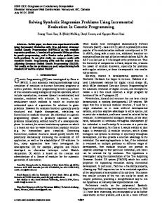
the query generation strategy proposed in Section 4. This elicitation strategy indeed consists in asking agents whether they approve or not some solutions found during the search; these solutions are obviously dependent on the branching strategy. For comparison, we also consider the interactive branch and bound procedure (named Random hereafter) that differs from IAS only on the branching strategy as follows: the next node to be explored and the next variable to be instantiated are both selected at random. For both branching strategies, we compute the maximum regret (MR) attached to the incumbent (using Proposition 6) each time an agent answers an approval query during the resolution. Recall that this regret gives an upper bound on the regret of choosing the incumbent instead of any other solution in terms of approval scores. Whenever this value equals zero, the incumbent is necessarily an approval winner. Regrets are here expressed on a normalized scale assigning value 1 to the initial maximum regret (computed before collecting any preference information) and value 0 when the maximum regret is 0. Figure 2 shows the results obtained by averaging over 30 runs.

Figure 3. Maximum regret attached to the incumbent at each step of the branch and bound procedures (p = 15, d = 0.5, n = 30).

6

Figure 2. Maximum regret attached to the incumbent with respect to the total number of queries (p = 12, d = 0.4, n = 30).

In Figure 2, we can see that the maximum regret reduces much more quickly with IAS than with Random. For instance, after 240 queries (i.e. 8 queries per agent) on average, the regret of choosing the incumbent instead of any true approval winner is under 10% of the initial regret, whereas it remains above 65% with the random branching strategy. Hence, the elicitation strategy seems to be much more informative using our regret-based branching strategy instead of the random branching strategy. Finally, we estimate the performance of IAS as an anytime algorithm by computing the maximum regret attached to the incumbent at each iteration step of IAS. This regret indeed provides a guarantee on the gap to optimality at any step of the branch and bound procedure. For comparison, we consider here also the random branch and bound procedure (named Random). The results reported in Figure 3 are obtained by averaging over 30 runs. We observe that the maximum regret decreases much more quickly with IAS than with Random, as the number of iteration steps increases. For instance, after 200 iteration steps on average, the maximum regret is under 10% with our procedure while remaining above 70% for the random strategy. Moreover, we observe that this regret drops drastically from the very beginning of IAS. This shows that IAS provides (very quickly) a good solution before the end of the search.

CONCLUSION

We have presented a new approach for incremental approval voting on combinatorial domains, illustrated on the knapsack problem. The first specificity of this approach is to exploit compact numerical representations of individual preferences (additive utilities) to propose more efficient elicitation sequences. Thus, learning that agent i approves or not solution x is no longer an isolated preference information; it induces a constraint on the utility space possibly reducing the set of weak-orders consistent with the observed preferences. This contributes to derive implicitly other approval judgements on other knapsacks, which saves many preference queries. The second specificity of our approach is to interleave preference elicitation and search. This makes it possible to elicit preferences on a combinatorial set implicitly defined with a twofold benefit in view of winner determination: on the one hand, working on partial instances of feasible solutions in the search tree facilitates the identification of relevant queries and relieves the elicitation burden. On the other hand, the search is earlier focused on the relevant part of the solution space due to the integration of new preference information at decisive steps of the search algorithm, which saves a significant part of the computational effort. This enables to solve large instances for which the systematic elicitation of all approval statements is not feasible. We see several directions to extend this work. The first one is to relax the additivity of individual utilities so as to be able to model interactions between items. In this line, it seems natural to use generalized additive utilities functions (GAI) that could also be elicited incrementally [10]. Another direction would be to consider alternative voting rules using possibly more information than approval statements. For example, positional scoring rules may be worth investigating under the assumption that individual preferences are representable by additive utilities. This is a challenging issue because, when preferences are only partially known, the ranges of possible ranks in individual rankings is generally too large to be decisive.

ACKNOWLEDGEMENTS We wish to thank J´erˆome Lang for stimulating discussions during the preparation of this paper. This work is supported by the ANR project 14-CE24-0007-01- Cocorico-CoDec.

REFERENCES [1] Haris Aziz, Markus Brill, Vincent Conitzer, Edith Elkind, Rupert Freeman, and Toby Walsh, ‘Justified representation in approval-based committee voting’, in Proceedings of AAAI’15, pp. 784–790, (2015). [2] Haris Aziz, Serge Gaspers, Joachim Gudmundsson, Simon Mackenzie, Nicholas Mattei, and Toby Walsh, ‘Computational aspects of multiwinner approval voting’, in Proceedings of AAMAS’15, pp. 107–115, (2015). [3] Nawal Benabbou and Patrice Perny, ‘Incremental Weight Elicitation for Multiobjective State Space Search’, in Proceedings of AAAI’15, pp. 1093–1099, (2015). [4] Nawal Benabbou and Patrice Perny, ‘On possibly optimal tradeoffs in multicriteria spanning tree problems’, in Proceedings of ADT’15, pp. 322–337, (2015). [5] Nadja Betzler, Arkadii Slinko, and Johannes Uhlmann, ‘On the computation of fully proportional representation’, Journal of Artificial Intelligence Research, 475–519, (2013). [6] Craig Boutilier, Ioannis Caragiannis, Simi Haber, Tyler Lu, Ariel D Procaccia, and Or Sheffet, ‘Optimal social choice functions: A utilitarian view’, Artificial Intelligence, 227, 190–213, (2015). [7] Craig Boutilier, Relu Patrascu, Pascal Poupart, and Dale Schuurmans, ‘Constraint-based Optimization and Utility Elicitation using the Minimax Decision Criterion’, Artifical Intelligence, 170(8–9), 686–713, (2006). [8] Steven J. Brams and Peter C. Fishburn, ‘Approval voting’, The American Political Science Review, 72(3), 831–847, (1978). [9] Felix Brandt, Vincent Conitzer, Ulle Endriss, J´erˆome Lang, and Ariel D. Procaccia, Cambridge University Press, 2016. In press. [10] Darius Braziunas and Craig Boutilier, ‘Minimax regret based elicitation of generalized additive utilities’, in Proceedings of UAI’07, pp. 25–32, (2007). [11] Ioannis Caragiannis and Ariel D Procaccia, ‘Voting almost maximizes social welfare despite limited communication’, Artificial Intelligence, 175(9), 1655–1671, (2011). [12] Urszula Chajewska, Daphne Koller, and Ronald Parr, ‘Making rational decisions using adaptive utility elicitation’, in Proceedings of AAAI’00, pp. 363–369, (2000). [13] John R Chamberlin and Paul N Courant, ‘Representative deliberations and representative decisions: Proportional representation and the Borda rule’, American Political Science Review, 77(03), 718–733, (1983). [14] Lihi Naamani Dery, Meir Kalech, Lior Rokach, and Bracha Shapira, ‘Reaching a joint decision with minimal elicitation of voter preferences’, Information Sciences, 278, 466–487, (2014). [15] Ning Ding and Fangzhen Lin, ‘Voting with partial information: what questions to ask?’, in Proceedings of AAMAS’13, pp. 1237–1238, (2013). [16] Edith Elkind, Piotr Faliszewski, Piotr Skowron, and Arkadii Slinko, ‘Properties of multiwinner voting rules’, in Proceedings of AAMAS’14, pp. 53–60, (2014). [17] M. Gelain, M. S. Pini, F. Rossi, K. B. Venable, and T. Walsh, ‘Elicitation strategies for soft constraint problems with missing preferences: Properties, algorithms and experimental studies’, Artificial Intelligence Journal, 174(3-4), 270–294, (2010). [18] Meir Kalech, Sarit Kraus, and Gal A. Kaminka, ‘Practical voting rules with partial information’, Autonomous Agents and Multi-Agent Systems, 22(1), 151–182, (2010). [19] D Marc Kilgour, ‘Approval balloting for multi-winner elections’, in Handbook on approval voting, 105–124, Springer, (2010). [20] Kathrin Konczak and J´erˆome Lang, ‘Voting procedures with incomplete preferences’, in Proceedings of IJCAI-05 Multidisciplinary Workshop on Advances in Preference Handling, volume 20, (2005). [21] J´erˆome Lang, Maria Silvia Pini, Francesca Rossi, Domenico Salvagnin, Kristen Brent Venable, and Toby Walsh, ‘Winner determination in voting trees with incomplete preferences and weighted votes’, Autonomous Agents and Multi-Agent Systems, 25(1), 130–157, (2012). [22] Tyler Lu and Craig Boutilier, ‘Budgeted social choice: From consensus to personalized decision making’, in Proceedings of IJCAI’11, volume 11, pp. 280–286, (2011). [23] Tyler Lu and Craig Boutilier, ‘Robust approximation and incremental elicitation in voting protocols’, in Proceedings of IJCAI’11, pp. 287– 293, (2011). [24] Tyler Lu and Craig Boutilier, ‘Multi-winner social choice with incomplete preferences’, in Proceedings of IJCAI’13, pp. 263–270, (2013).

[25] Reshef Meir, Ariel D Procaccia, Jeffrey S Rosenschein, and Aviv Zohar, ‘Complexity of strategic behavior in multi-winner elections.’, Journal of Artificial Intelligence Research (JAIR), 33, 149–178, (2008). [26] Burt L Monroe, ‘Fully proportional representation’, American Political Science Review, 89(04), 925–940, (1995). [27] Joel Oren and Brendan Lucier, ‘Online (budgeted) social choice’, Proceedings of AAAI’14, 1456–1462, (2014). [28] Richard F Potthoff and Steven J Brams, ‘Proportional representation broadening the options’, Journal of Theoretical Politics, 10(2), 147– 178, (1998). [29] Ariel D Procaccia and Jeffrey S Rosenschein, ‘The distortion of cardinal preferences in voting’, in Proceedings of the Tenth International Workshop on Cooperative Information Agent, 317–331, Springer, (2006). [30] Ariel D Procaccia, Jeffrey S Rosenschein, and Aviv Zohar, ‘On the complexity of achieving proportional representation’, Social Choice and Welfare, 30(3), 353–362, (2008). [31] Piotr Skowron, Piotr Faliszewski, and J´erˆome Lang, ‘Finding a collective set of items: From proportional multirepresentation to group recommendation’, in Proceedings of AAAI’15, pp. 2131–2137, (2015). [32] Piotr Skowron, Lan Yu, Piotr Faliszewski, and Edith Elkind, ‘The complexity of fully proportional representation for single-crossing electorates’, Theoretical Computer Science, 569, 43–57, (2015). [33] T. Wang and C. Boutilier, ‘Incremental Utility Elicitation with the Minimax Regret Decision Criterion’, in Proceedings of IJCAI-03, pp. 309– 316, (2003). [34] Lirong Xia and Vincent Conitzer, ‘Determining possible and necessary winners given partial orders’, Journal of Artificial Intelligence Research (JAIR), 41, 25–67, (2011).