PHYSICAL REVIEW E 72, 041909 共2005兲
Solving the advection-diffusion equations in biological contexts using the cellular Potts model Debasis Dan,* Chris Mueller, Kun Chen, and James A. Glazier† Biocomplexity Institute and Department of Physics, Indiana University, 727 E. 3rd Street, Swain Hall West 159, Bloomington, Indiana 47405-7105, USA 共Received 26 April 2005; published 10 October 2005兲 The cellular Potts model 共CPM兲 is a robust, cell-level methodology for simulation of biological tissues and morphogenesis. Both tissue physiology and morphogenesis depend on diffusion of chemical morphogens in the extra-cellular fluid or matrix 共ECM兲. Standard diffusion solvers applied to the cellular potts model use finite difference methods on the underlying CPM lattice. However, these methods produce a diffusing field tied to the underlying lattice, which is inaccurate in many biological situations in which cell or ECM movement causes advection rapid compared to diffusion. Finite difference schemes suffer numerical instabilities solving the resulting advection-diffusion equations. To circumvent these problems we simulate advection diffusion within the framework of the CPM using off-lattice finite-difference methods. We define a set of generalized fluid particles which detach advection and diffusion from the lattice. Diffusion occurs between neighboring fluid particles by local averaging rules which approximate the Laplacian. Directed spin flips in the CPM handle the advective movement of the fluid particles. A constraint on relative velocities in the fluid explicitly accounts for fluid viscosity. We use the CPM to solve various diffusion examples including multiple instantaneous sources, continuous sources, moving sources, and different boundary geometries and conditions to validate our approximation against analytical and established numerical solutions. We also verify the CPM results for Poiseuille flow and Taylor-Aris dispersion. DOI: 10.1103/PhysRevE.72.041909
PACS number共s兲: 87.10.⫹e, 02.70.Uu, 05.10.⫺a, 47.11.⫹j
I. INTRODUCTION
Advection-diffusion equations 共ADE兲 describe a broad range of natural phenomena. They occur in diverse fields including physics 关1兴, chemistry 关2兴, biology, geology 关3,4兴, and even in migration and epidemiology 关5兴. They describe the flow 共deterministic兲 and the spread 共stochastic兲 of a density 共of a chemical, heat, charge兲 which a fluid or deformable solid carries. The simplest ADE is
n ជ n, = D2n − ជ · ⵜ t
共1兲
where n is the density of the transported substance, D its diffusion constant 共here assumed uniform in space兲, and ជ is the velocity field. The velocity field in turn couples to the pressure field of the medium through the Navier-Stokes equations. Though we can solve the problem analytically in steady state with simple boundary conditions, most physically relevant ADEs appear within sets of nonlinear coupled equations or with nontrivial boundary conditions where analytical solutions are not possible 关6兴. Hence a vast literature exists on how to solve ADEs. Most solvers use either finite difference 共FD兲 or finite element 共FE兲 关7兴 schemes. Besides these deterministic approaches, several schemes use LatticeBoltzmann 共LB兲 methods 关8兴 like Flekkoy’s method 关9兴, Dawson’s method, 关10兴, and the moment-propagation method 关11兴. ADEs in general are difficult to solve in the absence of separation of diffusion and advection time scales or in the presence of moving boundaries. Most lattice-based
*Electronic address:
[email protected] †
Electronic address:
[email protected]
1539-3755/2005/72共4兲/041909共10兲/$23.00
methods locally refine the grid during solution to avoid instabilities. Moreover, explicit LB methods require time averaging of the torque to avoid instabilities 关12兴. Hence the computational cost of both LB and deterministic methods shoots up. Nonstaggered FD grids may show griddecoupling instabilities 关12兴. Also, all explicit methods require consideration of the general stability constraints from linear analysis, most notably the Neumann diffusive criterion linking the time step and the square of the grid size. In this paper we try to address the problems associated with incorporating advection diffusion in biologically motivated, multiscale simulations, specifically those which use the cellular Potts model 共CPM兲 to model cell behaviors. Diffusion of morphogens and flow of extra-cellular matrix 共ECM兲 are crucial to many biological phenomena, including wound healing, morphogenesis, e.g., during mesenchymal condensation or gastrulation 关13兴 and the immune response where cells emerge from the microvasculature and migrate toward sites of inflammation to kill bacteria, other pathogens, and cancer. The generic mechanisms common to all these processes are changes in cell velocities 共chemotaxis兲 or/and differentiation in response to the temporal and spatial variations of chemical morphogens. Other classic examples of diffusion-driven morphogenesis involve Turing instabilities. Turing instabilities arise due to different diffusion rates of two or more reacting chemicals resulting in competition between activation by a slow-diffusing chemical 共activator兲 and inhibition by a faster chemical 共inhibitor兲. Pattern formation during morphogenesis due to Turing instabilities is a subject by itself 关14兴. Besides chemotaxis, the formation and rate of extension of pseudopods which crucially depends on convective mass transport 关15,16兴 also influences cell motility. Hydrodynamic shear can also increase cell-cell adhesion efficiency by in-
041909-1
©2005 The American Physical Society
PHYSICAL REVIEW E 72, 041909 共2005兲
DAN et al.
creasing the number of binding receptors. Shear has a profound effect on neutrophil-platelet adhesion and neutrophil aggregation, key events in acute coronary syndromes like arterial thrombosis 共关17兴兲. Extensive work has shown that both fluid shear amplitude and shear exposure time modulate the interactions between polymorphonuclear leukocytes and colon carcinoma cells 关18兴. Gene expression and protein synthesis in endothelial cells also change upon application of arterial shear stresses 关19兴. In a prominent example, fluid shear allows optimal L-selectin-mediated leukocyte rolling only above a minimum threshold shear rate 关20兴. Hence multicellular modeling tools have to properly account for the advection-diffusion: Diffusion influencing the spatial and temporal distribution of chemical morphogens, advection controlling the rates of cell collisions, deformation, receptorligand bond formation 关21兴, adhesion, and enhanced mixing of chemical morphogens. Simulations of the development of multicellular organisms take diverse mathematical approaches: continuum FEbased models 关22兴 of reaction diffusion which consider cell density as a continuous variable 关23兴, hybrid models like E-cell 关24兴 and cellular automaton approaches 关25兴. Glazier and Graner developed the cell-level CPM, an extension of the energy-based large-Q Potts model, for organogenesis simulations 关26兴. The basic CPM explains how surface binding energies drive cell movement and models cell sorting from an initial random distribution into different patterns depending on the cell adhesion coefficients at homotypic, heterotypic, and cell-medium boundaries 关27兴. It also provides a platform on which to build simulations of a wide range of biological experiments by including additional mechanisms like directed active movement due to external fields, e.g., chemotaxis to a chemical field gradient, gravity, or cell polarity. CPM applications include modeling mesenchymal condensation 关25,28,29兴, the complete life-cycle of Dictyostelium discoideum 关30兴, tumor growth 关31兴, vascular development 关32兴, immune response, and limb growth 关33兴. Unlike the simple Turing mechanism where cells have no feedback on the chemical field, most CPM implementations include this feedback which can give rise to completely different patterning from the Turing mechanism. In the CPM, patterns can arise under the influence of a single chemical field 关13兴 due to cell movement, biased by gradients in cellcell adhesion and cell-ECM binding, which is impossible in Turing mechanism. This unique mechanism also differs from chemotaxis, which requires long-range cell movement 关28兴. All existing CPM implementations suffer from four main limitations: 共1兲 They do not include viscous dissipation explicitly. Instead dissipation arises from the MetropolisBoltzmann energy-minimization dynamics. This implicit dissipation makes viscosity hard to calculate or control. 共2兲 They do not explicitly describe force transduction through cells, which arises through the volume constraint and surface constraint 共if used兲 of the Hamiltonian. 共3兲 Aggregates of cells modeled with an ordinary CPM Hamiltonian are highly overdamped. Modeling the ECM or fluid as an array of generalized cells using the normal CPM produces a flow resembling the overdamped flow of biological fluid but this fluid slips at solid surfaces and exerts no shear force unlike a normal fluid. An alternative approach which describes the
fluid as a single, large, unconstrained generalized cell produces nonlocal movement. Moreover, it cannot advect chemicals or transmit shear forces. 共4兲 The CPM has no intrinsic concept of rigid-body motion. We will describe an algorithmic solution to this last problem, which makes the CPM look more like a FE simulation, in a future paper. All of these problems result from the CPM spins being tied to the underlying lattice, rather than to objects they describe. The solution in each case is to adopt a FE approach suited to the CPM, which takes the behavior off lattice. Applying standard off-lattice methods in the CPM has inherent problems. Since in the CPM cell movement occurs by boundary fluctuations, connecting normal FE fluid solvers to the CPM at surfaces requires local grid refinement during cell movement to avoid numerical instabilities. Hence its computational cost is high. To introduce advection diffusion in the CPM correctly and efficiently, we propose an off-lattice scheme consistent and in harmony with the CPM algorithm. We subdivide the ECM into small fluid particles having the normal properties of generalized cells like differential adhesivity, a surface constraint and a volume constraint. The fluid particles carry chemical morphogens and we assume the concentrations are uniform inside them. Diffusion occurs between neighboring fluid particles by local averaging rules which approximate the Laplacian. Spin flips in the CPM occur only at the boundaries of the cells or particles. A force on the fluid in any direction due to pressure gradients or external forces biases the probability of spin flips and generates directed motion 关34兴. We introduce viscosity into the CPM by explicitly including in the Hamiltonian including a relativevelocity constraint between the neighboring fluid particles. This scheme allows us to solve the ADEs and generates the creeping flow of a highly viscous fluid. In most biologically relevant regimes 共e.g., E. Coli in water兲, we encounter low Reynolds number 共Re兲 flow ⬃10−5, with the typical diffusion coefficient of chemical morphogens being ⬃10−4 m2 / s. Thus the Peclet number 共defined as R / D, where R , , D are typical size of the system, the typical fluid velocity, and diffusion coefficient, respectively兲 is as low as ⬃10−2 关35兴. We explicitly exclude blood flow in the circulatory system, where Re numbers 共hence inertia兲 can be quite large and where specialized solution techniques already exist. Since most CPM simulations do not demand high precision, sophisticated methods like mimetic finite difference 关36兴 become a computational bottleneck without many advantages. On the other hand, our ADE scheme is very stable, with spatial resolution equal to the mean diameter of the fluid particles, which are much smaller than the simulated biological cells. Our scheme seamlessly integrates into the main Monte Carlo loop of the CPM simulation and boundary conditions like absorbing boundaries or no-flux boundaries are simple to implement. More-over our offlattice scheme does not require remeshing. We discuss these issues in detail below. This paper mainly focuses on the validity and utility of the CPM ADE solver. Section II briefly describes the CPM along with the diffusion and advection scheme. Section III discusses various cases, including diffusion from two point sources, a continuous source, and a moving source with ei-
041909-2
PHYSICAL REVIEW E 72, 041909 共2005兲
SOLVING THE ADVECTION-DIFFUSION EQUATIONS…
ther reflecting or absorbing boundary conditions and the flow profile in Poisueille’s flow. Section IV outlines future directions in developing the ADE scheme. We will address in a future paper certain additional conditions, flow with inertia, effects of low or high Peclet numbers, constitutive properties of the fluid phase, etc. As we have stated before, ours method provides flexibility and efficiency in the biologically relevant regime of low Peclet and Reynolds numbers and where high numerical accuracy is not crucial.
II. MODEL
The Potts model is an energy-based, lattice cellularautomaton 共CA兲 model equivalent to an Ising model with more than two degenerate spin values. We typically use a cubic lattice with periodic or fixed boundary conditions in each direction. We use third or fourth nearest neighbor interactions to reduce lattice-anisotropy induced alignment and pinning. Each lattice site in the Potts model has a spin value. The energy, or Hamiltonian sums the interaction energies of these spins, according to predefined rules. In single-spin dynamics 共like Metropolis dynamics兲 the spin lattice evolves toward its equilibrium state by minimizing the interaction energy through spin flips. Multispin dynamics like Kawasaki dynamics are also possible. Though the original Potts model studies focuses on equilibrium properties, it can also model quasiequilibrium dynamical properties 关37兴. Using deterministic schemes for spin flips, patterns often stick in local minima. Finite-temperature Monte Carlo schemes circumvent this problem. These schemes accept a spin flip with temperature dependent Boltzmann or modified Boltzmann probability if the configuration encounters a potential barrier 共a greater energy after the spin flip than before兲 关37兴. We pick a target lattice site at random and one of its alien neighbors, also selected at random and attempt to flip the target spin to the value of the selected neighbor. In the modified Metropolis algorithm we employ, if the spin flip would produce a change in energy ⌬H, we accept the change with probability P given by P共⌬H兲 =
再
exp共− ⌬H/T兲 if ⌬H ⬎ 0, 1
otherwise,
冎
共2兲
where T is the fluctuation temperature. T controls the rate of acceptance of the proposed move. For very large T, all the moves are accepted and the dynamics is a random walk in the absence of barriers, i.e., interaction energies included in the Hamiltonian are effectively zero producing a disordered phase. For very small values of T the dynamics is deterministic and can trap in local minima. We choose T as the median value of the distribution of ⌬H, which is below the order-disorder phase transition temperature. All of our results are very robust with respect to a variation of T. S. Wong has recently shown that optimizing the dynamics of the modified Metropolis algorithm requires changes to the acceptance probability in Eq. 共2兲 关38兴. However, we do not implement these changes here. Our unit of time is Monte Carlo sweep 共MCS兲, where 1MCS= L3 spin flip attempts, L being the system size.
FIG. 1. A typical cell configuration in CPM. The bold lines denote cell boundary.
The CPM adapts the Potts model to the context of biology. A CPM cell is a collection of lattice sites with same spin value 共or index兲 i. Each cell has a unique spin 共see Fig. 1兲. Cells may also have additional characteristics, e.g., a type . Links between different sites with spins define cell boundaries. So cells have both volume and a surface area. The volume, area, and radius relations are highly non-Euclidean for small cells. The CPM Hamiltonian contains a variable number of terms. The interaction between pairs of biological cells involves an adhesive or repulsive interfacial energy. This interfacial energy is precisely the Potts energy, the sum of the interactions of neighboring unlike spins, across a link. Each mismatched link contributes a cell-type dependent binding energy per unit area J共 , ⬘兲, where and ⬘ are the type of cells on either side of the link. In the CPM the effective cell-cell interaction energy is Eadhesion =
兺
共i,j,k兲,共l,m,n兲neighbors
J关共i,j,k兲, 共l,m,n兲兴
⫻兵1 − ␦关共i,j,k兲,共l,m,n兲兴其,
共3兲
where ␦共⬘,兲 = 1 if ⬘ = , otherwise ␦共⬘,兲 = 0. At any time t, a cell, of type has a volume 共 , t兲 and surface area s共 , t兲. The volume is simple to define, 共0兲 = 兺i,j,k␦关0,共i,j,k兲兴, whereas surface area is more complex, since it depends on the interaction range of the lattice, s共0兲 = 兺i,j,k␦共0,i,j,k兲兺i⬘,j⬘,k⬘兵1 − ␦关共i,j,k兲,共i⬘,j⬘,k⬘兲兴其, where 共i , j , k兲 and 共i⬘ , j⬘ , k⬘兲 are neighboring lattice sites. Each cell has an effective volume elasticity, and target volume target共 , t兲. Larger values of , produce less compressible 2 cells. We typically choose target ⬎ other constraint energies. This compressibility makes little difference in low Reynolds number flow but makes pattern evolution less stiff. We also define a membrane elasticity s and a target surface area starget共 , t兲 to maintain the generalized shape of the cells. The energy contributions due to surface and volume fluctuations are Esurface = s关s共,t兲 − starget共,t兲兴2 ,
共4兲
Evolume = 关共,t兲 − target共,t兲兴2 .
共5兲
We can extend the Hamiltonian to include a uniform exជ , acting on all cells by including the term ternal force F
041909-3
PHYSICAL REVIEW E 72, 041909 共2005兲
DAN et al.
Eforce = −
Fជ · rជ i,j,k关1 − ␦共i,j,k兲,共l,m,n兲兴, 兺 共ijk兲,共lmn兲neighbors
共6兲
where rជ ijk is the position vector at the lattice site 共i , j , k兲. Previous CPM applications often treated fluid or ECM as a single large cell with no constraints. Here we take the coarse-grained approach to describe ECM. We assume the ECM consists of hypothetical fluid cells 共which we call particles to avoid confusion with the modeling of biological cells兲 having all the characteristic interactions and constraints of regular CPM cells. The volume constraint and the surface tension determine the elastic nature of the fluid. The fluid particles can move with respect to one another like a regular CPM cell via spin flips. Thus, local pressure developed due to movement or enlargement of actual biological cells will translate into motion of the surrounding ECM. This fluid motion causes advection and mixing along with molecular diffusion of chemical morphogens. We restrict consideration to the highly overdamped viscous world that most biological cells experience, so our fluid particles lack inertia. We also restrict to situations where the velocity of movement is much less than the velocity of sound, which is one lattice unit per MCS. We now introduce a relative velocity constraint between the cells/particles which faithfully captures the effects of shear due to the viscosity of the medium. In the CPM, velocity is a cell property defined as the displacement of the center of mass of the cell per MCS. Since the velocity gradient terms in the direction of the flow 共e.g., ui / xi兲 are the rate of change of volume 关40兴 which Eq. 共5兲 already includes, we need to keep only the contributions of cross terms of the form 共ui / x j兲2. In an incompressible fluid 共 · u = 0兲 the cross terms are the dissipation energy per unit volume 关6兴. In the CPM we model this term as Eviscosity = viscosity兺 兺 Sij i
j
共Vix − V jx兲2 d2ij
冑
共y i − y j兲2 + 共zi − z j兲2 d2ij
+ cyclic permutation of 共x,y,z兲,
共7兲
where the j’s are the indices of cells neighboring the ith cell and dij = 冑共xi − x j兲2 + 共y i − y j兲2 + 共zi − z j兲2 is the distance between the centers of cell i and cell j. Vix is the xˆ-component of the velocity of the ith cell. Since the cells are of irregular shape, we further weight the energy penalty by the cells common contact area Sij. We ensure that the cells are simply connected by using local connectivity checks during spin flip attempts. viscosity corresponds to the viscosity coefficient in the Navier-Stokes equations. has dependence on other system parameters like J, volume, and surface. The net Hamiltonian including fluids is then H = Eadhesion + Esurface + Evolume + Eviscosity .
共8兲
fluid particles configuration; C共xជ , t兲 / t = D2C共xជ , t兲, where we have assumed that the diffusion constant D is constant and isotropic. Including an anisotropic or spatially varying D is a trivial extension of our method. We assume that the fluid particles carry chemical morphogens, whose distribution is uniform over a given fluid particle. Equivalently we can associate the chemical concentration with the center of mass of the particles and think of the diffusion as taking place between them 共a FE view兲. Because the shape and volume of the fluid particles are irregular, their centers of mass do not correspond to lattice points. We then need a numerical scheme for diffusion among fluid particles. Few existing algorithms solve diffusion on a random or irregular lattice. The more sophisticated and accurate ones are computationally expensive 关36兴. We use a naive iterated Euler method, which is fast and stable and reproduces different biological experiments with good qualitative and fair quantitative accuracy. We could of course, use a more elaborate scheme, if necessary. We locally average the concentration among the particle’s nearest neighbors. The particle neighbors change as the fluid flows. We approximate the Laplacian 2C共rជ , t兲 关where C共rជ , t兲 is the chemical concentration and rជ is the center of mass coordinate of a fluid particle兴 by 关39兴 D2C j共t兲 ⬃ D
兺 i next to j
关Ci共rជ ,t兲 − C j共rជ ,t兲兴 , R2
共9兲
where R is the average radius of the fluid particles assuming N ជ , t兲 is the V1/3 them to be spherical 关R = 共兺i=1 i 兲 / N兴, and Ci共r concentration in nearest neighbor fluid particles. We use R2 instead of 兩rជ i − rជ j兩2 to avoid Neumann instability. We can update the concentration once or multiple times per MCS depending on the diffusion coefficient of the chemical morphogen. D along with the number of concentration updates per MCS controls the diffusion constant. For larger diffusion coefficients we update the diffusion step multiple times per MCS. For typical chemical morphogens like cAMP the diffusion constants are ⬃10−4 m2 / s, corresponding to a spread of 3冑2 . ⫻ 10−4 m共0.04 m兲 per MCS. The typical lattice spacing in our CPM corresponds to 0.1– 1.0 m, hence a fluid particle has a width of ⬃0.3– 3.0 m. Therefore a very small amount of chemical needs to diffuse among adjacent fluid particle per MCS. In fact, for most practical purposes we need at most one diffusion step per five to ten MCS. Both reflecting and constant concentration 共zero concentration is absorbing兲 boundaries are simple to implement. For reflecting boundary condition we exclude from the exchange of concentration 关Eq. 共9兲兴 any particle whose boundary is reflecting. For absorbing boundary condition 共constant concentration兲, we define the particles whose boundaries are absorbing to always have zero concentration. The algorithm handles moving boundaries automatically and conserves chemical concentration, unlike many other methods. III. RESULTS AND DISCUSSION
A. Diffusion scheme
A. Poiseuille flow
Since the motion of the fluid particles takes care of advection, we need only to solve the diffusion on the current
We first discuss simulating Poiseuille flow of a viscous fluid in a cylindrical tube with rigid walls under a uniform
041909-4
PHYSICAL REVIEW E 72, 041909 共2005兲
SOLVING THE ADVECTION-DIFFUSION EQUATIONS…
FIG. 2. 共Color online兲 共a兲 Velocity profile in a cylindrical flow under gravity and its fit to the analytical solution. 共b兲 Velocity profile across a diameter of the tube with error bars, the bold segment along the xˆ direction denotes the width of a fluid particle.
force field 共body force兲 using the CPM. We consider a cylindrical tube with a circular cross section of radius 18 lattice units and length 200 lattice units with periodic boundary condition along the length. Each fluid particle has an average volume of 64 lattice points. Our CPM AD scheme works for small forces when the fluid particles remain simply connected. Figure 2 plots the ensemble averaged 共50 different initial configurations兲 cross-sectional profile of the viscous ជ flow at x = 150 and t = 2000 MCS with a small force F = 0.05xˆ applied on all the fluid particles. The flow is in the x direction only. The profile is parabolic as expected. We also show its fit to the analytical solution V共r兲 = F / 4R2关1 − 共r / R兲2兴, where is the viscosity 共a fitting parameter兲, R = 18 is the radius of the cylinder, and r is the distance from the axis of the cylinder. What is surprising is the excellent agreement 共an error of ⬍5% with the analytical result despite the coarseness兲 of the simulation 共only 9 particles across the diameter兲. All lattice points inside a fluid particle have the same velocity, so regions where the shapes of the fluid particles are regular for most ensembles will produce plateaux in the velocity profile. Since in the CPM, the velocity of fluid particles is the center of mass velocity, a lattice point touching a boundary wall will have a small nonzero velocity as the center of mass of
the corresponding particle lies in the interior 共slip boundary兲. Since the energy contribution of the constraints near a boundary wall dominates the external applied force and the Monte Carlo temperature, boundary particles are more regular in shape than interior particles. This regularity holds in all ensembles, hence the rms error in the velocity near a boundary wall is small as shown in Fig. 3共b兲 and the velocity just near the boundary in Fig. 2 has a small plateau. Reducing the size of the fluid particles compared to the typical length scales of the flow reduces these anomalies. Increasing viscosity increases the viscosity coefficient . A future paper will study the relation between and , Monte Carlo temperature, fluid particle size, etc. We shall also show additional biologically relevant hydrodynamic flows. We next verify our diffusion scheme under various biologically relevant conditions. CPM models using the modified finite temperature Metropolis algorithm have diffusion due to the movement of the CPM cells themselves which adds to the diffusion of chemical morphogens. However for most CPM simulations, e.g., a temperature 0.1 and other parameter values used throughout this paper, the diffusion coefficient of the CPM cells is ⬃10−4 pixel2/MCS, which is much smaller than the typical diffusion coefficient of ⬃0.1 that we treat in this paper. Hence for pure diffusion in a static medium the fluid is effectively fixed. Besides the concentra-
FIG. 3. 共a兲 The absolute error between the analytical solution Vanalytical and the CPM simulation Vsimulation at x = 150. 共b兲 The rms error of over 50 ensembles. 041909-5
PHYSICAL REVIEW E 72, 041909 共2005兲
DAN et al.
FIG. 4. 共Color online兲 Symbols denote chemical profile projected on the x axis 共summing in the Y and Z directions兲 at t = 50, 100, and 200 MCS for reflecting barriers at x = 0 and 100 denoted by symbols. The solid line is a fit to the exact solution using the fitting parameter D. The inset shows variations in D with time, due to coarse graining and the initial sharp distribution.
tion profile of the diffusing chemical in a medium, diffusion in the presence of boundaries, and moving source is crucially important in biology. We show that the results of our simple CPM diffusion from CPM agree very well with corresponding analytical calculations or finite element results. We also briefly discuss the validity of our method for diffusion in Poiseuille flow. The four cases we discuss below employ fluid particles with a target volume target = 27, unless we mention otherwise. The lattice has 100⫻ 100⫻ 100 sites. We equilibrate and quench to remove any disconnected cells which the finite-temperature equilibration produces 关27兴. In our model a chemical source at a given lattice point gives all lattice points which belong to the fluid particle containing that chosen point the same concentration. We apply one diffusion step per MCS. The first three cases are for static fluids. B. Two sources with reflecting and absorbing boundaries
We consider two point sources at 15, 50, 50 and 50, 50, 50 with initial concentrations 共at t = 0兲 of 5 and 10, respec-
tively. The chemicals diffuse from these instantaneous sources. The bounding planes of the cube are reflecting. Figure 4 plots the corresponding one-dimensional diffusion profile projection 共with no ensemble average兲 after elapsed times t = 50, 100, 200 MCS, and fitted to the exact solution C共x,t兲 = 10.0/ 冑 共4Dt兲共exp关−共x − x1兲 + exp关−共2L1 − x − x1兲
2兴/4Dt
2兴/4Dt
+ exp关−共2L2 − x − x1兲
2兴/4Dt
兲
2兴/4Dt
兲,
关−共x − x2兲2兴/4Dt
+ 5.0/ 冑 共4Dt兲共exp + exp关−共2L1 − x − x2兲
2兴/4Dt
+ exp关−共2L2 − x − x2兲
D being a fit parameter. Here L1 and L2 are the coordinates of the two reflecting boundaries and x1 and x2 are the coordinates of the instantaneous sources. The diffusion profile matches very well at all times, even near the boundaries. The maximum relative error 共compared to the exact solution兲 at t = 50 MCS is 5%, again, surprisingly good for such a coarse simulation. We discuss errors in detail for absorbing boundary conditions in the next paragraph. The inset shows the variation of the diffusion coefficient calculated from fitting to
FIG. 5. 共Color online兲 Chemical profile projected on the x axis from diffusion of two instantaneous point sources for an absorbing barrier at x = 0 and x = 100 for t = 70, 100, and 200 MCS. The inset shows the variation of D with fluid particle volume on a log scale.
041909-6
PHYSICAL REVIEW E 72, 041909 共2005兲
SOLVING THE ADVECTION-DIFFUSION EQUATIONS…
FIG. 6. 共Color online兲 Relative error along the x lattice direction for an absorbing barrier.
the exact solution as a function of time. Though the diffusion constant should remain constant with time, we observe a 5–6 % variation from the asymptotic value at small times due to the sharp initial distribution producing structures smaller
than the fluid particle scale of our coarse-grained scheme. We also studied the variation of the diffusion coefficient D as a function of the target volume of the fluid particles. D is constant for variations over one order of magnitude of the
FIG. 7. 共Color online兲 Chemical profile cross section along z = 40, 50, and 60 in the presence of a cylindrical reflecting barrier with axis along the xˆ direction and rectangular cross section. The sources with initial concentration 5 and 10 are placed at 50, 40, 40 and 50, 60, 60. The inset shows 2D projection of the profile. The lower figure shows a two-dimensional projection obtained from finite element calculations. The concentration decreases as we go away from the center contours 共yellow lines兲.
041909-7
PHYSICAL REVIEW E 72, 041909 共2005兲
DAN et al.
FIG. 8. 共Color online兲 CPM simulation of the chemical profile from a moving source 共the other two coordinates integrated out兲 at t = 300 MCS. The solid line denotes the fit to Eq. 共10兲. The inset shows a two-dimensional projection of the simulation, where red denotes the highest chemical concentration and black the lowest.
target volume of the fluid particles as shown in the inset to Fig. 5. Figure 5 also shows the chemical profile for an absorbing barrier at x = 0 and x = 100. The figures show that the diffusion coefficient for both reflecting and absorbing barriers cases is same. Hence for a wide range of fluid particle volumes, our CPM ADE algorithm faithfully reproduces diffusion from two point sources. Figure 6 plots the relative error as a function of position at different times. As mentioned in the last paragraph the sharp distribution at the initial time produce errors large compared to later time, i.e., if we ignore the large errors in the tail 共as the magnitude of concentration is extremely small in the tails兲 the relative error at t = 150 is ⬍5% whereas at t = 500 it is ⬍0.5%. In the actual biological situation, cells secrete chemical morphogens over their whole membrane surface and hence such singular cases of high point concentration of chemical rarely occur. C. Two sources with a reflecting obstacle inside the medium
Since biological cells can be impermeable to many chemical morphogens, they can act as reflecting boundaries within the fluid medium. We check this situation for the simple test case of a cylindrical barrier with rectangular cross section
关15⫻ 15, pixels centered at 共50, 50, 50兲 and the axis along the x direction兴 within the fluid medium. As in the previous case, we place two point sources near the two opposite corners of the rectangle at 共50, 40, 40兲 and 共50, 60, 60兲. We recover the same diffusion coefficient as in the previous case. Figure 7 plots the one-dimensional cross section of the diffusion profile at three different z positions. Along z = 40 and 60 the barrier is absent and the diffusion is merely the superposition of that from the two sources. Along z = 50 we see the effect of the reflecting barrier. The inset on the right side shows the concentration profile obtained from a finite element calculation for this situation which matches very well with the CPM concentration profile in the left inset. D. Moving continuous source
Moving cells often secrete morphogens. Hence we correctly simulate cells’ chemotactic response to secreted chemicals only if we faithfully reproduce diffusion from moving sources. To test our simulation we assign an arbitrary fluid particle a constant concentration C0 共continuous source兲 and uniform velocity along the x direction. We keep the source sufficiently distant from the boundary to avoid bound-
FIG. 9. 共Color online兲 Effective diffusion coefficient for mean flow velocities ¯ = 0.056, 0.028, and 0.016, respectively from top to the bottom curve. The solid lines show the analytical results corresponding to above mean velocities.
041909-8
PHYSICAL REVIEW E 72, 041909 共2005兲
SOLVING THE ADVECTION-DIFFUSION EQUATIONS…
FIG. 10. 共Color online兲 Cross-sectional profile 共xˆ-zˆ plane, y = 20兲 of chemical concentration at t = 500 MCS starting from an initial set of particles at x = 75 with uniform concentration; 共a兲 with no diffusion, 共b兲 with diffusion. Particles which move away from the plane in the yˆ direction cannot be seen in the figures.
ary effects. At t = 0 the source is at x = 35 and moves with velocity u = 0.04 pixel/MCS. We fit the CPM chemical profile projection in the x direction 共no ensemble average兲 with the 1D analytical solution
C共x,t兲 =
␣共x兲 = 关共x − x0兲2兴/共4D兲,
共10兲
 = u2/共4D兲,
共11兲
␥共x兲 = exp关共x − x0兲u/共2D兲兴,
共12兲
C0 ␥共x兲关exp共2冑␣共x兲兲兴Erfc 2
冉冑
␣共x兲 冑 + t t
冊 共13兲
冉
+ exp关− 2冑␣共x兲兴Erfc
冉冑
冊
␣共x兲 冑 − t . t
共14兲
+¯2R2 / 48D0. Here D0 is the diffusion coefficient in the absence of flow, ¯ is the average velocity, and R is the radius of the cylinder. Figure 9 shows our results where we have plotted the variation of effective diffusion coefficient with time 共in MCS兲 for different mean velocities. For the analytical results given in solid lines in Fig. 9, we use the mean velocity obtained from the fit of the velocity profile as shown in Fig. 2. Figure 10 shows snapshots of chemical profile after 500 MCS for D0 = 0 and D0 = 0.12. In this case, we start with a thin sheet of chemical in the x-z plane, at x = 75, i.e., all the particles at x = 75 have uniform concentration. We take a cut at y = 20 to see the evolved chemical profile. A detailed study of evolution of chemical profile, effect of embedded objects like sphere under both stationary and moving conditions will be reported in our future communication. IV. CONCLUSIONS
We check the qualitative agreement of the dispersion coefficient obtained using our CPM ADE solver for Poiseuille flow along the x direction 共described in Sec. III A兲 in a cylindrical geometry. We compare our result for an initial delta distribution of chemical in the middle of the tube. After an initial transient, so that the chemical reaches the boundary in the y and z directions, we compare the diffusion coefficient of chemical distribution along the x direction with the analytical result for the effective diffusion coefficient in Poiseuille flow along the cylinder axis, i.e., Deffective = D0
We have implemented fluid flow, advection, and diffusion in the framework of the CPM, avoiding the programming complexity and computational demands associated with implementing a finite-element or finite-difference NavierStokes simulation and interfacing it with the CPM lattice. We have used three biologically relevant test cases to verify our method. All our results for diffusion in the presence of boundaries or moving sources agree very well with corresponding analytical or finite-element solutions. The errors in our scheme are large if we try to probe far below the diffusion time scale or the fluid particle length scale, but the results are qualitatively correct. Thus we must be cautious when applying this scheme to large Pe number flows. The requirement that fluid particles remains connected, limits the method to low Re. However, since most biological mechanisms operate at low Re our CPM ADE solver is appropriate for many cell-level simulations.
关1兴 C. R. Nugent, W. M. Quarles, and T. H. Solomon, Phys. Rev. Lett. 93, 218301 共2004兲; J. D. Seymour, J. P. Gage, S. L. Codd, and R. Gerlach, ibid. 93, 198103 共2004兲; M. Leconte, J. Martin, N. Rakotomalala, and D. Salin, ibid. 90, 128302
共2003兲; B. F. Edwards, ibid. 89, 104501 共2002兲. 关2兴 A. Bancaud, G. Wagner, K. D. Dorfman, and J. L. Viovy Anal. Biochem. 77, 833 共2005兲. 关3兴 T. Yanagita and K. Kaneko, Phys. Rev. Lett. 78, 4297 共1997兲.
Figure 8 shows that the CPM diffusion agrees very well with the analytical solution. The diffusion coefficient obtained from the fit is D = 0.29. E. Taylor-Aris dispersion in Poiseuille flow
041909-9
PHYSICAL REVIEW E 72, 041909 共2005兲
DAN et al. 关4兴 J. M. Keller and M. L. Brusseau, Environ. Sci. Technol. 37, 3141 共2003兲; T. E. McKone and D. H. Bennett, ibid. 37, 3123 共2003兲. 关5兴 G. J. Gibson, C. A. Gilligan, and A. Kleczkowski, Proc. R. Soc. London, Ser. B 266, 1743 共1999兲; J. T. Truscott and C. A. Gilligan, Proc. Natl. Acad. Sci. U.S.A. 100, 9067 共2003兲. 关6兴 T. E. Faber, Fluid Dynamics for Physicists 共Cambridge University Press, Cambridge, England, 1995兲. 关7兴 P. M. Gresho and R. L. Sani, Incompressible Flow and the Finite Element Method 共Wiley, New York, 2000兲; W. Hundsdorfer and J. G. Verwer, Numerical Solution of TimeDependent Advection-Diffusion-Reaction Equations, Springer Series in Computational Mathematics 共Springer, New York, 2003兲. 关8兴 Y. H. Qian, D. D’Humieres, and P. Lallemand, Europhys. Lett. 17, 479 共1992兲. 关9兴 E. G. Flekkoy, Phys. Rev. E 47, 4247 共1993兲. 关10兴 S. P. Dawson, S. Chen, and G. D. Doolean, J. Chem. Phys. 98, 1514 共1993兲. 关11兴 C. P. Lowe and D. Frenkel, Physica A 220, 251 共1995兲; R. H. Merks et al., J. Comput. Phys. 183, 563 共2002兲. 关12兴 J. C. Anthony, J. Fluid Mech. 271, 285 共1994兲. 关13兴 W. Zeng, G. L. Thomas, S. A. Newman, and J. A. Glazier, Mathematical Modeling and Computing in Biology and Medicine, 5th ESMTB Conference 2002, edited by V. Capasso 共Societ Editrice Esculapio, Bologna, 2003兲. 关14兴 A. M. Turing, Philos. Trans. R. Soc. London, Ser. B 237, 266 共1952兲; A. Taylor, Prog. React. Kinet. 27, 247 共2002兲. 关15兴 D. V. Zhelev, A. M. Alteraifi, and D. Chodniewicz, Biophys. J. 87, 688–695 共2004兲. 关16兴 H. C. Berg and P. M. Tedesco, Proc. Natl. Acad. Sci. U.S.A. 72, 3235 共1975兲. 关17兴 M. H. Kroll, J. D. Hellums, L. V. McIntire, A. L. Schafer, and J. L. Moake, Blood 88, 1525 共1996兲. 关18兴 S. Jadhav and K. Konstantopoulos, Am. J. Physiol.: Cell Physiol. 283, C1133 共2002兲. 关19兴 M. U. Nollert, N. J. Panaro, and L. V. McIntire, Ann. N.Y. Acad. Sci. 665, 94 共1992兲; P. F. Davies, Physiol. Rev. 75, 519 共1995兲. 关20兴 E. B. Finger, K. D. Puri, R. Alon, M. B. Lawrence, U. H. von
关21兴 关22兴 关23兴 关24兴 关25兴
关26兴 关27兴 关28兴 关29兴 关30兴
关31兴 关32兴 关33兴
关34兴 关35兴 关36兴 关37兴 关38兴 关39兴 关40兴
041909-10
Andrian, and T. A. Springer, Nature 共London兲 379, 266 共1996兲. A. D. Taylor, S. Neelamegham, J. D. Hellums, C. W. Smith, and S. I. Simon, Biophys. J. 71, 3488 共2004兲. M. Pavlin, N. Pavselj, and D. Miklavcic, IEEE Trans. Biomed. Eng. 49, 605 共2002兲. H. G. E. Hentschel, J. A. Glazier, and S. A. Newman, Proc. R. Soc. London, Ser. B 271, 1713 共2004兲. S. Kikichi et al., Neural Networks 16, 1389 共2003兲. M. S. Alber, A. Kiskowski, J. A. Glazier, and Y. Jiang, Math. Syst. Theory Biology, Communication, and Finance 134, 1 共2003兲. F. Graner and J. A. Glazier, Phys. Rev. Lett. 69, 2013 共1992兲. J. A. Glazier and F. Graner, Phys. Rev. E 47, 2128 共1993兲. W. Zeng, G. L. Thomas, and J. A. Glazier, Physica A 341, 482 共2004兲. M. Zajac, G. L. Jones, and J. A. Glazier, Phys. Rev. Lett. 85, 2022 共2000兲. S. Maree, Ph.D. thesis University Utrecht, 2000; A. F. MarAee and P. Hogeweg, Proc. Natl. Acad. Sci. U.S.A. 98, 3879 共2001兲. Emma Stott, N. F. Britton, J. A. Glazier, and M. Zajac, Math. Comput. Modell. 30, 183 共1999兲. R. M. H. Merks, S. A. Newman, and J. A. Glazier, Lect. Notes Comput. Sci. 3305, 425 共2004兲. R. Chaturvedi, J. A. Izaguirre, C. Huang, T. Cickovski, P. Virtue, G. Thomas, G. Forgacs, M. Alber, G. Hentschel, S. A. Newman, and J. A. Glazier, Lect. Notes Comput. Sci. 2659, 39 共2003兲. Y. Jiang, Cellular Pattern Formation, Ph.D. dissertation, University of Notre Dame, 1998. E. M. Purcell, Am. J. Phys. 45, 3 共1977兲. J. Braun and M. Sambridge, Nature 共London兲 376, 655 共1995兲. M. E. J. Newman and G. T. Barkema, Monte Carlo Methods in Statistical Physics 共Oxford University, New York, 1999兲. S. Wong, Ph.D. thesis, Notre Dame University, 2004. J. D. Murray, Mathematical Biology, Vol. 1 共Springer-Verlag, Berlin, 2002兲. E. M. Lifsihtz and L. D. Landau, Fluid Mechanics 共Butterworth-Heinemann, Oxford, 1987兲.