Dec 3, 2014 - Basic Idea: âsweepâ through S performing a full backup operation on each s. â· A few different methods exist. E.g.: â» Policy Iteration and.
Solving the Bellman Optimality Equations: Basic Methods AI & Agents for IET Lecturer: S Luz http://www.scss.tcd.ie/~luzs/t/cs7032/
December 3, 2014
1
The basic background & assumptions I
Environment is a finite MDP (i.e. A and S are finite).
I
MDP’s dynamics defined by transition probabilities:
I
and expected immediate rewards,
I
Goal: to search for good policies π
I
Strategy: use value functions to structure search:
The basic background & assumptions I
Environment is a finite MDP (i.e. A and S are finite).
I
MDP’s dynamics defined by transition probabilities: a 0 Pss 0 = P(st+1 = s |st = s, at = a)
I
and expected immediate rewards, Rass 0 = E {rt+1 |st = s, at = a, st+1 = s 0 }
I
Goal: to search for good policies π
I
Strategy: use value functions to structure search: X a a 0 V ∗ (s) = max Pss 0 [Rss 0 + γV ∗ (s )] a
Q ∗ (s, a) =
X s0
s0 a a ∗ 0 0 Pss 0 [Rss 0 + γ max Q (s , a )] 0 a
or
Overview of methods for solving Bellman’s equations
I
Dynamic programming: I I
3
well-understood mathematical properties... ...but require a complete and accurate model of the environment
Overview of methods for solving Bellman’s equations
I
Dynamic programming: I I
I
Monte Carlo (simulation methods): I I I
3
well-understood mathematical properties... ...but require a complete and accurate model of the environment conceptually simple no model required... ...but unsuitable for incremental computation
Overview of methods for solving Bellman’s equations
I
Dynamic programming: I I
I
Monte Carlo (simulation methods): I I I
I
conceptually simple no model required... ...but unsuitable for incremental computation
Temporal difference methods I I I
3
well-understood mathematical properties... ...but require a complete and accurate model of the environment
also require no model; suitable for incremental computation... ... but mathematically complex to analyse
Dynamic programming
I
I
Basic Idea: “sweep” through S performing a full backup operation on each s. A few different methods exist. E.g.: I I
I
Policy Iteration and Value Iteration.
The building blocks: I I
Policy Evaluation: how to compute V π for an arbitrary π. Policy Improvement: how to compute an improved π given V π .
Policy Evaluation
The task of computing V π for an arbitrary π is known as the prediction problem. I As we have seen, a state-value function is given by
I
V π (s)
= Eπ {Rt |st = s} = Eπ {rt+1 + γV π (st+1 )|st = s} X X = π(s, a) Pssa 0 [Rass 0 + γV π (s 0 )] a
I
s0
a system of |S| linear equations in |S| unknowns (the state values V π (s))
Iterative Policy evaluation
I
Consider the sequence of approximations V0 , . . . V π .
I
Choose V0 arbitrarily and set each successive approximation accommodation to the Bellman equation: Vk+1 (s) ← Eπ {rt+1 + γVk (st+1 )|st = s} X X a a 0 ← π(s, a) Pss 0 [Rss 0 + γVk (s )]
I
6
“Sweeps”: V0 → V1 → . . . ↑ ↑
(1)
s0
a
→ Vk ↑
→ Vk+1 . . . ↑
→ Vπ ↑
Iterative Policy Evaluation Algorithm 1 2 3
Initialisation : f o r ( each s ∈ S ) V (s) ← 0
4 5 6 7 8 9 10 11 12 13
IPE ( π ) /∗ π : p o l i c y to repeat ∆ ← 0 Vk ← V f o r ( e a c hPs ∈ S/{sP terminal } ) V (s) ← a π(s, a) s 0 Pssa 0 [Rass 0 + γVk (s 0 )] ∆ ← max(∆, |Vk (s) − V (s)|) until ∆ < θ /∗ θ > 0 : a return V I
7
be
e v a l u a t e d
small /∗
∗/
c o n s t a n t π
V ≈V
NB: alternatively one could evaluate V π in place (i.e usnig a single vector V to store all values and update it directly).
∗/ ∗/
An example: an episodic GridWorld
I
Rewards of −1 until terminal state (shown in grey) is reached
I
Undiscounted episodic task:
actions
8
1
2
3
4
5
6
7
8
9
10
11
12
13
14
r = −1 on all transitions
Policy Evaluation for the GridWorld
I
Iterative evaluation of Vk for equiprobable random policy π:
Policy Evaluation for the GridWorld
I
Iterative evaluation of Vk for equiprobable random policy π: 0.0 0.0 0.0 0.0 0.0 0.0 0.0 0.0
V0 →
0.0 0.0 0.0 0.0 0.0 0.0 0.0 0.0
9
Policy Evaluation for the GridWorld
I
Iterative evaluation of Vk for equiprobable random policy π:
V0 →
0.0 0.0 0.0 0.0
0.0 -1.0 -1.0 -1.0
0.0 0.0 0.0 0.0
-1.0 -1.0 -1.0 -1.0
0.0 0.0 0.0 0.0 0.0 0.0 0.0 0.0
9
V1 →
-1.0 -1.0 -1.0 -1.0 -1.0 -1.0 -1.0 0.0
Policy Evaluation for the GridWorld
I
Iterative evaluation of Vk for equiprobable random policy π:
V0 →
0.0 0.0 0.0 0.0
0.0 -1.0 -1.0 -1.0
0.0 -1.7 -2.0 -2.0
0.0 0.0 0.0 0.0
-1.0 -1.0 -1.0 -1.0
-1.7 -2.0 -2.0 -2.0
0.0 0.0 0.0 0.0 0.0 0.0 0.0 0.0
9
V1 →
-1.0 -1.0 -1.0 -1.0 -1.0 -1.0 -1.0 0.0
V2 →
-2.0 -2.0 -2.0 -1.7 -2.0 -2.0 -1.7 0.0
Policy Evaluation for the GridWorld
I
Iterative evaluation of Vk for equiprobable random policy π:
V0 →
0.0 0.0 0.0 0.0
0.0 -1.0 -1.0 -1.0
0.0 -1.7 -2.0 -2.0
0.0 0.0 0.0 0.0
-1.0 -1.0 -1.0 -1.0
-1.7 -2.0 -2.0 -2.0
0.0 0.0 0.0 0.0 0.0 0.0 0.0 0.0 0.0 -2.4 -2.9 -3.0 -2.4 -2.9 -3.0 -2.9
V3 →
-2.9 -3.0 -2.9 -2.4 -3.0 -2.9 -2.4 0.0
V1 →
-1.0 -1.0 -1.0 -1.0 -1.0 -1.0 -1.0 0.0
V2 →
-2.0 -2.0 -2.0 -1.7 -2.0 -2.0 -1.7 0.0
Policy Evaluation for the GridWorld
I
Iterative evaluation of Vk for equiprobable random policy π:
V0 →
0.0 0.0 0.0 0.0
0.0 -1.0 -1.0 -1.0
0.0 -1.7 -2.0 -2.0
0.0 0.0 0.0 0.0
-1.0 -1.0 -1.0 -1.0
-1.7 -2.0 -2.0 -2.0
0.0 0.0 0.0 0.0
V1 →
0.0 0.0 0.0 0.0
-1.0 -1.0 -1.0 0.0
0.0 -2.4 -2.9 -3.0
0.0 -6.1 -8.4 -9.0 -6.1 -7.7 -8.4 -8.4
-2.4 -2.9 -3.0 -2.9
V3 →
-1.0 -1.0 -1.0 -1.0
-2.9 -3.0 -2.9 -2.4 -3.0 -2.9 -2.4 0.0
V10 →
-8.4 -8.4 -7.7 -6.1 -9.0 -8.4 -6.1 0.0
V2 →
-2.0 -2.0 -2.0 -1.7 -2.0 -2.0 -1.7 0.0
Policy Evaluation for the GridWorld
I
Iterative evaluation of Vk for equiprobable random policy π:
V0 →
0.0 0.0 0.0 0.0
0.0 -1.0 -1.0 -1.0
0.0 -1.7 -2.0 -2.0
0.0 0.0 0.0 0.0
-1.0 -1.0 -1.0 -1.0
-1.7 -2.0 -2.0 -2.0
0.0 0.0 0.0 0.0
V1 →
0.0 0.0 0.0 0.0
-1.0 -1.0 -1.0 0.0
0.0 -2.4 -2.9 -3.0
0.0 -6.1 -8.4 -9.0
-2.9 -3.0 -2.9 -2.4 -3.0 -2.9 -2.4 0.0
V2 →
V10 →
-8.4 -8.4 -7.7 -6.1 -9.0 -8.4 -6.1 0.0
-2.0 -2.0 -2.0 -1.7 -2.0 -2.0 -1.7 0.0 0.0 -14. -20. -22.
-6.1 -7.7 -8.4 -8.4
-2.4 -2.9 -3.0 -2.9
V3 →
-1.0 -1.0 -1.0 -1.0
-14. -18. -20. -20.
V∞ →
-20. -20. -18. -14. -22. -20. -14. 0.0
Policy Improvement
I
Consider the following: how would the expected return change for a policy π if instead of following π(s) for a given state s we choose an action a 6= π(s)?
I
For this setting, the value would be:
Policy Improvement
I
Consider the following: how would the expected return change for a policy π if instead of following π(s) for a given state s we choose an action a 6= π(s)?
I
For this setting, the value would be: Q π (s, a) = Eπ {rt+1 + γV π (st+1 )|st = s, at = a} X a a π = Pss 0 [Rss 0 + γV (st+1 )] s0
I
So, a should be preferred iff Q π (s, a) > V π (s)
Policy improvement theorem
If choosing a 6= π(s) implies Q π (s, a) ≥ V π (s) for a state s, then the policy π 0 obtained by choosing a every time s is encoutered (and 0 following π otherwise) is at least as good as π (i.e. V π (s) ≥ V π (s)). 0 If Q π (s, a) > V π (s) then V π (s) > V π (s)
I
If we apply this strategy to all states to get a new greedy 0 policy π 0 (s) = arg maxa Q π (s, a), then V π ≥ V π
I
V π = V π implies that
0
0
V π (s) = max a
which is...
11
X s0
π 0 a a Pss 0 [Rss 0 + γV (s )]
Policy improvement theorem
If choosing a 6= π(s) implies Q π (s, a) ≥ V π (s) for a state s, then the policy π 0 obtained by choosing a every time s is encoutered (and 0 following π otherwise) is at least as good as π (i.e. V π (s) ≥ V π (s)). 0 If Q π (s, a) > V π (s) then V π (s) > V π (s)
I
If we apply this strategy to all states to get a new greedy 0 policy π 0 (s) = arg maxa Q π (s, a), then V π ≥ V π
I
V π = V π implies that
0
0
V π (s) = max a
X
π 0 a a Pss 0 [Rss 0 + γV (s )]
s0
which is... a form of the Bellman optimality equation.
11
Policy improvement theorem If choosing a 6= π(s) implies Q π (s, a) ≥ V π (s) for a state s, then the policy π 0 obtained by choosing a every time s is encoutered (and 0 following π otherwise) is at least as good as π (i.e. V π (s) ≥ V π (s)). π π π0 π If Q (s, a) > V (s) then V (s) > V (s)
I
If we apply this strategy to all states to get a new greedy 0 policy π 0 (s) = arg maxa Q π (s, a), then V π ≥ V π
I
V π = V π implies that
0
0
V π (s) = max a
I
11
X
a π 0 a Pss 0 [Rss 0 + γV (s )]
s0
which is... a form of the Bellman optimality equation. 0 Therefore V π = V π = V ∗
Improving the GridWorld policy
0.0 0.0 0.0 0.0 0.0 0.0 0.0 0.0 0.0 0.0 0.0 0.0 0.0 0.0 0.0 0.0
→
Improving the GridWorld policy
0.0 0.0 0.0 0.0
0.0 -1.0 -1.0 -1.0
0.0 0.0 0.0 0.0
-1.0 -1.0 -1.0 -1.0
0.0 0.0 0.0 0.0
-1.0 -1.0 -1.0 -1.0
0.0 0.0 0.0 0.0
-1.0 -1.0 -1.0 0.0
→
→
Improving the GridWorld policy
0.0 0.0 0.0 0.0
0.0 -1.0 -1.0 -1.0
0.0 0.0 0.0 0.0
-1.0 -1.0 -1.0 -1.0
0.0 0.0 0.0 0.0
-1.0 -1.0 -1.0 -1.0
0.0 0.0 0.0 0.0
-1.0 -1.0 -1.0 0.0
→
0.0 -1.7 -2.0 -2.0 -1.7 -2.0 -2.0 -2.0 -2.0 -2.0 -2.0 -1.7 -2.0 -2.0 -1.7 0.0
→
→
Improving the GridWorld policy
0.0 0.0 0.0 0.0
0.0 -1.0 -1.0 -1.0
0.0 0.0 0.0 0.0
-1.0 -1.0 -1.0 -1.0
0.0 0.0 0.0 0.0
-1.0 -1.0 -1.0 -1.0
0.0 0.0 0.0 0.0
-1.0 -1.0 -1.0 0.0
→
-1.7 -2.0 -2.0 -2.0
-2.4 -2.9 -3.0 -2.9
-2.0 -2.0 -2.0 -1.7
-2.9 -3.0 -2.9 -2.4
-2.0 -2.0 -1.7 0.0
→
0.0 -2.4 -2.9 -3.0
0.0 -1.7 -2.0 -2.0
→
-3.0 -2.9 -2.4 0.0
→
Improving the GridWorld policy
0.0 0.0 0.0 0.0
0.0 -1.0 -1.0 -1.0
0.0 0.0 0.0 0.0
-1.0 -1.0 -1.0 -1.0
0.0 0.0 0.0 0.0
-1.0 -1.0 -1.0 -1.0
0.0 0.0 0.0 0.0
-1.0 -1.0 -1.0 0.0
→
-1.7 -2.0 -2.0 -2.0
-2.4 -2.9 -3.0 -2.9
-2.0 -2.0 -2.0 -1.7
-2.9 -3.0 -2.9 -2.4
-2.0 -2.0 -1.7 0.0
→
0.0 -6.1 -8.4 -9.0 -6.1 -7.7 -8.4 -8.4 -8.4 -8.4 -7.7 -6.1 -9.0 -8.4 -6.1 0.0
→
0.0 -2.4 -2.9 -3.0
0.0 -1.7 -2.0 -2.0
→
-3.0 -2.9 -2.4 0.0
→
Improving the GridWorld policy
0.0 0.0 0.0 0.0
0.0 -1.0 -1.0 -1.0
0.0 0.0 0.0 0.0
-1.0 -1.0 -1.0 -1.0
0.0 0.0 0.0 0.0
-1.0 -1.0 -1.0 -1.0
0.0 0.0 0.0 0.0
-1.0 -1.0 -1.0 0.0
→
-1.7 -2.0 -2.0 -2.0
-2.4 -2.9 -3.0 -2.9
-2.0 -2.0 -2.0 -1.7
-2.9 -3.0 -2.9 -2.4
-2.0 -2.0 -1.7 0.0
→
0.0 -6.1 -8.4 -9.0
-3.0 -2.9 -2.4 0.0
→
0.0 -14. -20. -22.
-6.1 -7.7 -8.4 -8.4
-14. -18. -20. -20.
-8.4 -8.4 -7.7 -6.1
-20. -20. -18. -14.
-9.0 -8.4 -6.1 0.0
→
0.0 -2.4 -2.9 -3.0
0.0 -1.7 -2.0 -2.0
→
-22. -20. -14. 0.0
→
Putting them together: Policy Iteration π0
Putting them together: Policy Iteration eval
π0 −→
Putting them together: Policy Iteration eval
π0 −→ Vπ0
Putting them together: Policy Iteration eval
improve
π0 −→ Vπ0 −→
Putting them together: Policy Iteration eval
improve
π0 −→ Vπ0 −→ π1
Putting them together: Policy Iteration eval
improve
e
π0 −→ Vπ0 −→ π1 −→
Putting them together: Policy Iteration eval
improve
e
π0 −→ Vπ0 −→ π1 −→ Vπ1
Putting them together: Policy Iteration eval
improve
e
i
i
π0 −→ Vπ0 −→ π1 −→ Vπ1 −→ · · · −→
Putting them together: Policy Iteration eval
improve
e
i
i
π0 −→ Vπ0 −→ π1 −→ Vπ1 −→ · · · −→ π ∗
Putting them together: Policy Iteration eval
improve
e
i
i
e
π0 −→ Vπ0 −→ π1 −→ Vπ1 −→ · · · −→ π ∗ −→
Putting them together: Policy Iteration eval
improve
e
i
i
e
π0 −→ Vπ0 −→ π1 −→ Vπ1 −→ · · · −→ π ∗ −→ V ∗
Putting them together: Policy Iteration eval
improve
e
i
i
e
π0 −→ Vπ0 −→ π1 −→ Vπ1 −→ · · · −→ π ∗ −→ V ∗ 1 2 3
Initialisation : for all s ∈ S V (s) ← an a r b i t r a r y v ∈ R
4 5 6 7 8 9 10 11 12 13 14 15
Policy Improvement (π ) : do s t a b l e (π ) ← t r u e V ← IPE ( π ) f o r each s ∈ S b ← π(s) P a [Ra + γV (s 0 )] π(s) ← arg maxa s 0 Pss 0 ss 0 i f ( b 6= π(s) ) s t a b l e (π ) ← f a l s e w h i l e ( not s t a b l e (π ) ) return π
Other DP methods
I
Value Iteration: evaluation is stopped after a single sweep (one backup of each state). The backup rule is then: X a a 0 Vk+1 (s) ← max Pss 0 [Rss 0 + γVk (s )] a
I
s0
Asynchronous DP: back up the values of states in any order, using whatever values of other states happen to be available. I
On problems with large state spaces, asynchronous DP methods are often preferred
Generalised policy iteration
Value Iteration I
1 2 3
Potential computational savings over Policy Iteration in terms of policy evaluation
Initialisation : for all s ∈ S V (s) ← an a r b i t r a r y v ∈ R
4 5 6 7 8 9 10 11 12 13 14
15
Value I t e r a t i o n (π ) : repeat ∆ ← 0 f o r each s ∈ S v ← V (s) P a [Ra + γV (s 0 )] V (s) ← maxa s 0 Pss 0 ss 0 ∆ ← max(∆, |v − V (s)|) until ∆ < θ return determin Pi s t i ca π as . t . 0 π(s) = arg maxa s 0 Pss 0 [Rss 0 + γV (s )]
Summary of methods
full backups
sample backups
shallow backups
16
bootstrapping, λ
deep backups
Summary of methods Exhaustive search full backups
sample backups
shallow backups
16
bootstrapping, λ
deep backups
Summary of methods Dynamic programming
Exhaustive search
full backups
sample backups
shallow backups
16
bootstrapping, λ
deep backups
Monte Carlo Methods
I
Complete knowledge of environment is not necessary
I
Only experience is required Learning can be on-line (no model needed) or through simulated experience (model only needs to generate sample transitions.
I
I
I I
In both cases, learning is based on averaged sample returns.
As in DP, one can use an evaluation-improvement strategy. Evaluation can be done by keeping averages of: I I
Every Visit to a state in an episode, or of the First Visit to a state in an episode.
Estimating value-state functions in MC
The first visit policy evaluation method:
1 2 3 4
F i r s t V i s i t M C (π ) Initialisation : V ← arbitrary state values Returns(s) ← empty l i s t o f s i z e |S|
5 6 7 8 9 10 11
18
Repeat G e n e r a t e an e p i s o d e E u s i n g π For each s i n E R ← return f o l l o w i n g the f i s r t Append R t o Returns(s) V (s) ← mean(Returns(s))
occurrence of s
Example Evaluate the policy described below for blackjack [Sutton and Barto, 1998, section 5.1] I
Actions: stick (stop receiving cards), hit (receive another card)
I
Play against dealer, who has a fixed strategy (‘hit’ if sum < 17; ‘stick’ otherwise).
I
You win if your card sum is greater than the dealer’s without exceeding 21. States:
I
I I I
current sum (12-21) dealers showing card (ace-10) do I have a useable ace (can be 11 without making sum exceed 21)?
I
Reward: +1 for winning, 0 for a draw, -1 for losing
I
Policy: Stick if my sum is 20 or 21, else hit
MC value function for blackjack example
I
20
Question: compare MC to DP in estimating the value function. Do we know the the environment? The transition probabilities? The expected returns given each state and action? What does the MC backup diagram look like?
Monte Carlo control I
Monte Carlo version of DP policy iteration:
I
Policy improvement theorem applies: Q πk (s, πk+1 (s)) = Q πk (s, arg max Q πk (s, a)) a
= max Q πk (s, a) a
≥ Q πk (s, a) = V πk (s)
21
MC policy iteration (exploring starts)
1 2 3 4
I
As with DP, we have evaluation-improvement cycles.
I
Learn Q ∗ (if no model is available)
I
One must make sure that each state-action pair can be a starting pair (with probability > 0). MonteCarloES ( ) I n i t i a l i s a t i o n , ∀s ∈ S, a ∈ A : Q(s, a) ← a r b i t r a r y ; π(s) ← a r b i t r a r y Returns(s, a) ← empty l i s t o f s i z e |S|
5 6 7 8 9 10 11 12 13
22
R e p e a t u n t i l s t o p − c r i t e r i o n met G e n e r a t e an e p i s o d e E u s i n g π and e x p l o t i n g s t a r t s F o r e a c h (s, a) i n E R ← r e t u r n f o l l o w i n g t h e f i s r t o c c u r r e n c e o f s, a Append R t o Returns(s, a) Q(s, a) ← mean(Returns(s, a)) For each s i n E π(s) ← arg maxa Q(s, a)
Optimal policy for blackjack example I
23
Optimal policy found by MonteCarloES for the blackjack example, and its state-value function:
On- and off- policy MC control
I
MonteCarloES assumes that all states are observed an infinite number of times and episodes are generated with exploring starts I
24
For an analysis of convergence properties, see [Tsitsiklis, 2003]
I
On-policy and off-policy methods relax these assumptions to produce practical algorithms
I
On-policy methods use a given policy and �-greedy strategy (see lecture on Evaluative Feeback) to generate episodes.
I
Off-policy methods evaluate a policy while generating an episode through a different policy
On-policy control
25
Summary of methods
full backups
sample backups
shallow backups
26
bootstrapping, λ
deep backups
Summary of methods Exhaustive search full backups
sample backups
shallow backups
26
bootstrapping, λ
deep backups
Summary of methods Dynamic programming
Exhaustive search
full backups
sample backups
shallow backups
26
bootstrapping, λ
deep backups
Summary of methods Dynamic programming
Exhaustive search
full backups
Monte Carlo
sample backups
shallow backups
26
bootstrapping, λ
deep backups
References
Notes based on [Sutton and Barto, 1998, ch 4-6]. Convergence results for several MC algorithms are given by [Tsitsiklis, 2003]. Sutton, R. S. and Barto, A. G. (1998). Reinforcement Learning: An Introduction. MIT Press, Cambridge, MA. Tsitsiklis, J. N. (2003). On the convergence of optimistic policy iteration. The Journal of Machine Learning Research, 3:59–72.
27