Solving the Course Scheduling Problem Using Simulated ... - iyte

Solving the Course Scheduling Problem Using Simulated Annealing E. Aycan and T. Ayav Department of Computer Engineering ˙Izmir Institute of Technology Email: {esraaycan, tolgaayav}@iyte.edu.tr

Abstract— This paper tackles the NP-complete problem of academic class scheduling (or timetabling). The aim is to find a feasible timetable for the department of computer engineering ˙ in Izmir Institute of Technology. The approach focuses on simulated annealing. We compare the performance of various neighborhood searching algorithms based on so-called simple search, swapping, simple search-swapping and their combinations, taking into account the execution times and the final costs. The most satisfactory timetable is achieved with the combination of all these three algorithms. The results highlight the efficacy of the proposed scheme.

Keywords - course scheduling, simulated annealing, neighborhood searching I. I NTRODUCTION The University Course Timetabling Problem (UCTP) is a common problem that almost every university has to solve. The basic definition states that UCTP is a task of assigning the events of a university (lectures, activities, etc) to the various resources such as lecturers, classrooms and time slots. This is done by minimizing the violations of a predefined set of constraints. In other words, no teacher, no class or no room should appear more than once in any period of time. There are also other timetabling problems described in the literature such as examination timetabling, school timetabling, employee timetabling, etc.. All these problems share similar characteristics and they are similarly difficult to solve. The general university course timetabling problem is known to be NP-complete, as many of the subproblems are associated with additional constraints. The intention of this paper is to study course timetabling with special emphasis on department-based timetabling as a classical application area where various types of preferences need to be satisfied to obtain a feasible solution. Thus, it is focused on the solution techniques for course timetabling of ˙Izmir Institute of Technology Computer Engineering Department. In the following section, the course scheduling problem in the university is presented. This is done in two steps: We first describe the problem, then give some formal definitions. In section III, Simulated Annealing (SA) method is presented. Our approach is mainly based on SA, yet the performance of SA highly rely on the initial solution, neighborhood search and cooling process, as described in section III. We use constraint

programming for finding an initial solution and try various neighborhood search algorithms. The comparison results are demonstrated in section IV and related work is given in section V. Finally, we conclude the paper in section VI. II. C OURSE S CHEDULING P ROBLEM In the Department of Computer Engineering of ˙Izmir Institute of Technology, course scheduling has been performed by the senior staff members manually so far. However, solving the course scheduling problem by hand usually might fail to satisfy all the constraints. According to the definition of course scheduling, in order to obtain an appropriate solution, all hard constraints have to be satisfied, while trying to fulfill as many soft constraints as possible. As a case study, 2007 − 2008 Fall Semester is handled. This problem consists of 5 classes (including postgraduate classes) with 5 classrooms and a shared laboratory. In this case, any constraint related with classrooms is ignored such as capacity of the rooms or room availability, since each class has its own classroom in computer engineering department. Totally there are 20 lectures given by 8 instructors in this case study. Lecture durations can change between 3 and 5, but the lectures that take 5 time slots are divided as 3 slots for theoretical and 2 slots for laboratory lectures. Hence, the laboratory lessons are considered as a separate lesson of which duration is 2 time slots and they are assigned to the laboratory. There can be maximum 8 time slots for one day in the university, i.e., there are 40 time slots per week. By considering all these conditions, the hard constraints can be constructed as follows: C1 : Each instructor can take only one class at a time. C2 : Clashes must not occur between the lectures for students of one class. C3 : If any instructor has some requests that have to be satisfied, their demands must be fulfilled. C4 : If any class has to take lectures from other departments, the time slots that are given from those departments must be allowed to those lectures. C5 : All lectures must start and finish in the same day. The soft constraints taken into account are: C6 : The number of alternatives that students can attend should be maximized. C7 : The student conflicts between lectures should be minimized.

C8 : C9 :

Friday should be free for all classes. Preferences of instructors should be fulfilled.

The model of the case study problem is modeled according to the definition of constraint satisfaction problem. A constraint satisfaction problem is a triple (Z, D, C) where Z is a finite set of variables {x1 , x2 , · · · , xn }, D is a function which maps every variable in Z to a set of objects of arbitrary type, i.e., D : Z → finite set of objects (of any type). Dxi , the domain of xi , is taken as the set of objects mapped from xi by D. These objects are called possible values of xi and the set Dxi . C is a finite (possibly empty) set of constraints on an arbitrary subset of variables in Z. In other words, C is a set of sets of compound labels. Because course scheduling problem is a real life problem which has plenty of constraints, it is categorized under the optimization problem. Hence the triple definition of the constraint satisfaction problem (denoted by P) becomes quadruple (Z, D, C, F ) where F is the objective function that indicates the quality of the solution. Formally, we denote with cs(P) the solution of P by any constraint satisfaction method [1]. Similarly, we use sa(P) to denote the solution of P by simulated annealing. Starting from a good point for searching a feasible solution is a very critical step in simulated annealing. We use constraint satisfaction methods for an initial timetable satisfying all the hard constraints and some of the soft constraints. Subsequently for fine tuning, we use simulated annealing in order to optimize a given objective function, F . This optimization allows us to take into account the soft constraints more effectively. The model consists of a set of resources and a set of activities. The time slots can be assigned a constraint, either hard or soft; a hard constraint indicates that the slot is forbidden for any activity, a soft constraint indicates that the slot is not preferred. These constraints are called as time preferences. Time preferences can be assigned to each activity and each resource, which indicate forbidden and non preferable time slots [2]. The lectures are called activities in the timetabling model. Every activity is defined by its duration (expressed as a number of time slots), by time preferences, and by a set of resources. Activities require these set of resources. Resources also can be described by time preferences. Only one activity can use a resource at any time. Each resource can represent a teacher, a class, a classroom, or another special resource. The solution of the problem defined by the above model is a timetable where every scheduled activity has its assigned start time and a set of reserved resources needed for its execution. This timetable must satisfy all the hard constraints. According to this structure; 1) Every scheduled activity has all the required resources reserved. 2) Two scheduled activities cannot use the same resource at the same time. 3) No activity is scheduled into a time slot where the activity or some of its reserved resources has a hard constraint in the time preferences.

Furthermore, the number of violated soft constraints are tried to be minimized. III. S IMULATED A NNEALING M ETHOD The application of Simulated Annealing (SA) to the timetabling problem is relatively straight forward. The particles are replaced by elements. The system energy can be defined by the timetable cost for timetable modeling. An initial allocation is made in which elements are placed in a randomly chosen period. The initial cost and an initial temperature are computed. To determine the quality of the solution, the cost has a critical role in the algorithm just as the system energy role in the quality of a particle being annealed. The temperature is used to control the probability of an increase in cost and can be likened by the temperature of a physical particle [3]. The change in cost is the difference of two costs; one of them is the first cost that is before the perturbation and the second one is the cost after the randomly chosen element is changed of an activity. The element is moved if the change in cost is accepted, either because it lowers the system cost, or the increase is allowed at the current temperature. According to the timetabling problem model, the cost of removing an element usually consists of a class cost, an instructor cost and a room cost. SA is an iterative method and a typical SA algorithm accepts a new solution if its cost is lower than the cost of the current solution in each iteration. Even if the cost of the new solution is greater, there is a probability of this solution to be accepted. With this acceptance criterion it is then possible to climb out of a local minima. The SA algorithm we use, denoted with sa(P), can be seen in Fig. 1 [4]. Find a random initial solution s := s0 using cs(P) Select an initial temperature t := t0 > 0 Select a temperature reduction function α repeat repeat s := N eighborhoodSearching(s) δ := F (s ) − F (s) if((δ ≤ 0) or (exp(−δ/t) < rand[0, 1])) s := s endif until iteration count = nrep t := CoolingSchedule(t) until stopping condition is true Fig. 1.

Pseudo-code of the SA algorithm

One should note that several aspects of the SA algorithm are problem oriented. In the design of a good annealing algorithm, deciding about proper neighborhood structure, cost function and cooling schedule are of paramount importance. We only focus on neighborhood searching in this context. A. Neighborhood Searching In order to implement the SA algorithm a neighborhood structure must be defined. This is the key component of any simulated annealing method. In this study, three algorithms

are handled in different combinations. In each iteration of the algorithm, neighborhood searching is performed once to find out the next possible solution set. More explicitly, we utilize the following algorithms: 1) Simple Searching Neighborhood (SSN ): The first one of the neighbor algorithm is simple searching neighborhood. It randomly chooses one activity and one slot. The chosen slot is assigned as the start time of the selected activity (see Fig. 2). Please note that Slot(ac) depicts the starting slot of activity ac. 2) Swapping Neighborhoods (SW N ): The second algorithm selects randomly two activities and swaps their start times (see Fig. 3). 3) Simple Searching and Swapping Neighborhoods (S 3 W N ): This neighborhood searching algorithm chooses randomly two activities and two slots. These two slots are assigned as the start times of the randomly selected activities (see in Fig. 4). SSN() { ac := select random activity(); sl := select random time slot(); Slot(ac) := sl; } Fig. 2.

Pseudo-code of the SSN algorithm used in neighborhood searching.

SWN() { ac1 := select random activity1(); ac2 := select random activity2(); sl := Slot(ac1); Slot(ac1) := Slot(ac2); Slot(ac2) := sl; } Fig. 3. Pseudo-code of the SWN algorithm used in neighborhood searching.

S3 WN() { ac1 := select random activity1(); ac2 := select random activity2(); sl1 := select random time slot1(); sl2 := select random time slot2(); Slot(ac1) := sl1; Slot(ac2) := sl2; } Fig. 4. Pseudo-code of the S3 WN algorithm used in neighborhood searching.

B. Cost Calculation For the case of course scheduling, the cost calculation tries to show the influences of both the hard constraints and soft constraints. Penalty scores of both the hard constraints and soft constraints are presented below. Each constraint is defined by a penalty score function. The conditions that the timetable has penalties for hard constraints are:

1) If the activity slots are hard slots that violate the hard constraints of that activity; FC1 = w1

n 

Ti ,

(1)

i=1

where n is the number of activities, w1 is the weight and Ti is the number of time slots which are forbidden to the activities. 2) If the same instructor is assigned to two activities at the same time; FC2 = w2

n−1 

n 

Iij ,

(2)

i=1 j=i+1

where n is the number of activities, w2 is the weight, Iij is the number of instructors who give two lectures, i and j, at the same time. 3) If the same class is assigned to two activities at the same time; n−1 n   Cij , (3) FC3 = w3 i=1 j=i+1

where n is the number of activities, w3 is the weight, Cij is the number of classes which are given to two lectures, i and j, at the same time. 4) If the activity slots are separated into two days. (Each activity must start and finish in the same day). FC4 = w4

n 

Xi ,

(4)

i=1

where n is the number of activities, Xi is the number of time slots which are given to lectures i, it is a boolean variable which becomes true when the course is separated into two days and w4 is the weight. The conditions that the timetable has penalties for soft constraints are: 5) If the activity slots are soft slots that violates the soft constraints of which activity; FC5 = w5

n 

Yi ,

(5)

i=1

where n is the number of activities, Yi is the number of time slots which depends on preferences of instructors and w5 is the weight. It can be inferred soft slots either. 6) If there is any student conflict between the previously failed lectures that a student has to take, and the regular lectures that are yet to be taken. FC6 = w6

n−1 

n 

Sij ,

(6)

i=1 j=i+1

where n is the number of activities, Sij is the number of students who take two lectures of different classes, i and j, at the same time. If a student follows an irregular program, the lecture conflicts are minimized by this constraint. It is taken as a soft constraint, otherwise

course scheduling problems would be very strict and had no solution. To determine the student conflicts, all the information about the students and lectures are collected from the university’s database system so that any irregular situation can be identified. For instance, if a third year standing student has some unsatisfied courses from the second year, which conflict with the third year courses, these conflicts should be avoided. For hard constraints, the given penalties (wi ) must be very high, e.g., approximately ∞. For soft constraints, penalties can be chosen smaller, taking into account the priorities of the constraints. Therefore, the cost function F can be calculated as the sum of those hard and soft constraints, i.e., F = FC 1 + F C 2 + F C 3 + F C 4 + F C 5 + F C 6 .

(7)

C. Cooling Schedule We use geometric cooling schedule as the cooling function. In every nrep iterations, the next temperature is found by t := αt

(8)

where α is the reduction parameter for geometric cooling and calculated as, α = 1 − (ln(t) − ln(tf ))/Nmove

(9)

where t is the current temperature, tf is the final temperature and Nmove is a fixed value that affects the duration of the temperature decrease. The parameter of nrep is chosen as 3, which returns the best solution cost within an acceptable execution time. To determine nrep , several different values such as 1, 2, 3, 5, 6 and 10 are experimented. A rough initial temperature t0 is assigned 10000. This temperature is hot enough to allow moves to almost every neighborhood state, and the SA algorithm iteratively updates the temperature using the functional dependence between the starting acceptance probability χ0 (60% to 70%) and the starting temperature t0 . This functional dependence is as follows: χ0

= χ(δ1 , δn , δn+1 , · · · , δm , t0 ) n  = 1/m exp(−δi /t0 ) + (m − n)/n

(10)

i=1

where δi = F (si ) − F (s0 ), s0 is the initial solution, si is a neighbor solution of s0 , F is the cost function, m is the size of neighbor solution space. Initial temperature t0 is derived from the starting acceptance probability χ0 using the algorithm presented in [4]. For instance, in our settings, t0 is calculated as 5000. This algorithm has to be run only once before executing the SA algorithm.

TABLE I T HE EFFECT OF Nmove ON C OSTS AND E XECUTION TIMES . Nmove Execution time (sec) Cost

10

50

100

500

1000

3000

0.8 2018800

3 4100

6 3500

29 3300

60 3400

154 3300

different neighborhood searching algorithms are demonstrated. First, Table II compare three different algorithms presented in the previous sections, namely SSN , SW N and S 3 W N . According to the table, SSN provides the best result. Since SA is a heuristic method, several experiments should be done and the technique that returns the best result in an appropriate time should be chosen. Table III and IV show an hybrid approach. The former one considers three pairs in combination, i.e., SSN − SW N , SW N − S 3 W N and SSN −S 3 W N . The latter shows the case that three algorithms are used all together. This consists of two cases, A and B. In case A, all algorithms are executed sequentially in each iteration. In case B, they are executed in turn basis, which turns the best result among all these trials. Finally, in Fig. IV, TABLE II C OSTS AND EXECUTION TIMES WITH THREE NEIGHBORHOOD SEARCH ALGORITHMS .

Cost 3900

SSN CPU(sec) 29

Cost 9300

SWN CPU(sec) 40

Cost 4300

S3 WN CPU(sec) 34

TABLE III C OSTS AND EXECUTION TIMES WITH THE COMBINATIONS OF SN , SW N AND

SSN and SWN Cost CPU(sec) 3900 28

S3W N .

SSN and S3 WN Cost CPU(sec) 4900 27

SWN and S3 WN Cost CPU(sec) 3700 31

TABLE IV C OSTS AND E XECUTION TIMES WHEN SSN, SWN AND S3 WN ARE USED ALL TOGETHER . Case A (sequentially) Cost CPU(sec) 4100 87

Case B (in turn) Cost CPU(sec) 3600 28

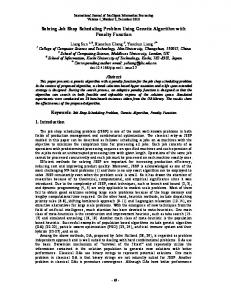
the cost change during the annealing (in case B) is illustrated. In the first phase, the initial cost obtained by cs(P) is 17600. After the annealing, the cost achieves its final value of 3600.

IV. E XPERIMENTAL R ESULTS In the experiments, we mainly focus on the comparisons of the neighborhood search algorithms. First, one can see the effect of Nmove on the total execution time of the SA algorithm and the final cost in Table I. In the rest of the tables, we use Nmove = 500 since it gives the most satisfactory results in terms of the final cost and execution time. Three

V. R ELATED W ORK Timetabling problem has been worked on over the years, so that many different solutions have been proposed. Precise and heuristic solution approaches for the school and university timetabling problem have been studied since the 1960s [5], [6], [7], [3], [8], [9], [10], [11], [12], [13], [2].

in the implementation of the SA algorithm. The stage of the hybrid approach may be integrated more fully, to yield a more powerful and robust algorithm. Another method for obtaining more quality results can be performing reheating techniques in simulated annealing. By reheating, one can get rid of hinging on local minima. TABLE V C OMPARISON OF THE TWO TIMETABLES PREPARED MANUALLY AND BY S IMULATED A NNEALING . Manually by the Staff 5011800 Fig. 5.

With Simulated Annealing 3600

Change of cost during the annealing process

If the history of the solution approaches are looked into, one can notice that various solving methods have been proposed for this problem. Operations Research literature has been extensively studied in building university timetables over the last 30 years. There are new solution techniques which have been evolving alongside the developments in mathematics and computer sciences. The methods for solutions vary from graph coloring to complex meta-heuristic algorithms, including Linear Programming formulations fitted to the specific problem at hand. Hertz [14] has applied Tabu Search techniques, Abramson [3] use simulated annealing and several authors like Burke et al. [8], Ross et al. [15] and Paechter et al. [16] have developed procedures based on variants of genetic algorithms. A different approach is Constraint Logic Programming, as Brailsford [12]. In recent years, hybrid methods become more popular and they are found more worthy to study on. The aim of the hybrid approach is to take the best ideas from one approach and incorporate them with other good ideas from other approaches. In spite of the shortcomings of the comparisons, the hybrid approaches still prove as promising algorithms. Hybridization has been proven to be very effective in the course timetabling literature [17], [18], [19]. VI. C ONCLUSION This paper presents simulated annealing mechanism for the course scheduling problem of the university’s computer engineering department. The approach is successfully realized by customizing the method for the application’s specific needs. The manually obtained timetable in the 2007-2008 fall term has a higher cost than the one obtained by SA method (see Table V). The method satisfies the hard constraints in the problem and finds out a feasible solution by means of exploiting a number of soft constraints. By utilizing three different neighborhood searching algorithms together with their combinations, the best result is achieved. For less solution time, the balance between solution quality and search time can be achieved through the predefined-time simulated annealing technique used in this SA algorithm. For a future work, the results of the experiments demonstrated in the previous section can be improved by some modifications

R EFERENCES [1] E. Tsang, Foundations of constraint satisfaction. London and San Diego: Academic Press, 1993. [2] T. Muller, “Constraint-based timetabling,” Ph.D. dissertation, Charles University, 2005. [3] D. Abramson, “Constructing school timetables using simulated annealing,” Management Science, vol. 37, no. 1, pp. 98–113, 1991. [4] T. Duong, “Combining constraint programming and simulated annealing on university exam timetabling,” Research Informatics Vietnam and Francophone, pp. 205–210, 2004. [5] M. Almond, “An algorithm for constructing university timetables,” Computer Journal, vol. 8, pp. 331–340, 1996. [6] A. Tripathy, “School timetabling, a case in large binary integer linear programming,” Management Science, vol. 30, pp. 1473–1489, 1984. [7] D. Werra, “An introduction to timetabling,” European Journal of Operation Research, vol. 19, pp. 151–162, 1985. [8] D. E. Edmund Burke and R. Weare, “A genetic algorithm based university timetabling system,” East-West International Conference on Computer Technologies in Education, vol. 1, pp. 35–40, 1994. [9] V. A. H Gunadhi and W. Yeong, “Automated timetabling using an object oriented scheduler,” Expert Systems with Applications, vol. 10, no. 2, pp. 243–256, 1996. [10] N. J. Christelle Guret and C. Prins, “Building university timetables using constraint logic programming,” In Practice and Theory of Automated Timetabling, pp. 130–145, 1996. [11] A. Schaerf, “A survey of automated timetabling,” Articifial Intelligence Review, vol. 13, no. 2, pp. 87–127, 1999. [12] C. N. P. S C Brailsford and B. M. Smith, “Constraint satisfaction problems: Algorithms and applications,” European Journal of Operational Research, no. 119, pp. 557–581, 1999. [13] S. Abdennadher and M. Marte, “University course timetabling using constraint handling rules,” Journal of Applied Artificial Intelligence, vol. 14, no. 4, pp. 311–326, 2000. [14] A. Hertz, “Finding a feasible course schedule using tabu search,” Discrete Appl. Math., vol. 35, no. 3, pp. 255–270, 1992. [15] D. Corne and P. Ross, Practice and Theory of Automated Timetabling, J. H. Kingston, Ed. Springer-Verlag, 1996, vol. 1153. [16] M. G. N. Ben Paechter, Andrew Cumming and H. Luchian, Practice and Theory of Automated Timetabling. Springer Berlin / Heidelberg, 1996, vol. 1153. [17] S. Abdullah and A. R. Hamdan, “A hybrid approach for university course timetabling,” International Journal of Computer Science and Network Security,, vol. 8, no. 8, 2008. [18] J. Thompson and K. Dowsland, “A robust simulated annealing based examination timetabling system,” Computers and Operations Research, vol. 25, pp. 637–648, 1998. [19] P. Kostuch, “The university course timetabling problem with a threephase approach.” International Conference on the Practice and Theory of Automated Timetabling (PATAT V), pp. 109–125, 2005.