SOM based data mining approach for discovery of ADSL usage profile Françoise Fessant, Fabrice Clérot R&D France Telecom 2, Avenue Pierre Marzin, 22307 Lannion
[email protected] [email protected] Résumé : The very rapid adoption of new applications by some segments of the ADSL customers may have a strong impact on the quality of service delivered to all customers. This makes the segmentation of ADSL customers according to their network usage a critical step both for a better understanding of the market and for the prediction and dimensioning of the network. Relying on a “bandwidth only" perspective to characterize network customer behaviour does not allow the discovery of usage patterns in terms of applications. In this paper, we shall describe how data mining techniques applied to network measurement data can help to extract some qualitative and quantitative knowledge. Mots-clés : Self organizing maps, aggregate usage profile, knowledge representation.
1 Introduction Broadband access for home users and small or medium business and especially ADSL (Asymmetric Digital Subscriber Line) access is of vital importance for telecommunication companies, since it allows them to leverage their copper infrastructure so as to offer new value added broadband services to their customers. The market for broadband access has several strong characteristics : – there is a strong competition between the various actors, – although the market is now very rapidly increasing, customer retention is important because of high acquisition costs, – new applications or services may be picked up very fast by some segments of the customers and the behaviour of these applications or services may have a very strong impact on the quality of service delivered to all customers (and not only those using these new applications or services). Two well-known examples of new applications or services with possibly very demanding requirements in term of bandwidth are peer-to-peer file exchange systems and audio or video streaming.
CAp 2007
The above characteristics explain the importance of an accurate understanding of the customer behaviour and a better knowledge of the usage of broadband access. The notion of “usage" is slowly shifting from a “bandwidth only" perspective to a much broader perspective which involves the discovery of usage patterns in terms of applications or services. The knowledge of such patterns is expected to give a much better understanding of the market and to help anticipate on the adoption of new services or applications by some segments and allow the deployment of new resources before its effect hits all the customers. Usage patterns are most often inferred from polls and interviews which allow an indepth understanding but are difficult to perform routinely, suffer from the small size of the sampled population and cannot be easily extended to the whole population or correlated with measurements (Anderson et al., 2002) and (Lelong & Beaudouin, 2001). “Bandwidth only" measurements are performed routinely on very large scale by telecommunication companies (Clément et al., 2002) but do not allow much insight into the usage patterns since the volumes generated by different applications can span many orders of magnitude. In this paper, we report another approach to the discovery of broadband customers’ usage patterns by directly mining network measurement data. After a description of the data used in the study and their acquisition process, we illustrate, through several analyses and data mining techniques, the ability of our approach to give an accurate insight in terms of applications or services usages patterns while being highly scalable and deployable. We focus on two complementary aspects of customers’ usages : usage of types of applications and customers’ daily traffic ; these analyses suppose to observe the data at several levels of description (some part of this work has already been presented in (Fessant et al., 2007)).
2 Network measurements and data description 2.1 Probes measurements The network measurements are performed on ADSL customer traffic by means of a proprietary network probe working at the SDH (Synchronous Digital Hierarchy) level between the Broadband Access Server (BAS) and the Digital Subscriber Line Access Multiplexer (DSLAM). This on-line probe allows to read and store all the relevant fields of the ATM (Asynchronous Transfer Mode) cells and of the IP/TCP headers. From now, 9 probes equip the network ; they observe about 18000 customers non-stop (a probe can observe about 2000 customers on a physical link). Once the probe in place, data collection is performed automatically. A detailed description of the probe architecture can be found in (François, 2002).
2.2 Data description For the study reported here, we gathered one month of data, on one site, for about two thousand customers. The data give the volumes of data exchanged in the upstream and downstream directions of twelve types of applications (web, peer-to-peer, ftp, news,
ADSL customer segmentation with SOMs
mail, db, control, games, streaming, chat, others and unknown) sampled for each 6 minutes window for each customer. Most of the types of applications correspond to a group of well known TCP ports, except the last two which relate to some well known but “obscure" ports (others) or dynamic ones (unknown). Since much of peer-to-peer traffic uses dynamic ports, peer-to-peer applications are recognized from a list of application names by scanning the payloads at the application level and not by relying on the wellknown ports only. This is done transparently for the customers ; no other use is made of such data than statistical analysis.
3 Customers segmentation according to their usage of the network The aim of this study is a better understanding of the customers’ usage patterns in terms of types of applications - precisely, what we are looking for is a set of combinations of applications (a pattern such as a "large e-mail user and small peer-to-peer user"). To achieve this task we have defined the activity of a customer by his total monthly traffic on the twelve types of applications (both for the upstream and the downstream).
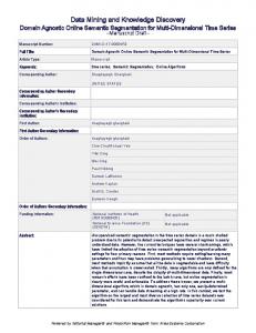
3.1 Data pre-processing : the use of rank statistics Figure 1 plots the distribution of the total monthly traffic on the applications (all days and customers included) for one site in September 2003 (the volumes are given in bytes). About 90 percent of the traffic is due to peer-to-peer, web and unknown applications and all the monitored sites show a similar distribution. 12
5
x 10
P2P
4.5
upstream traffic
4
downstream traffic
3
6 7 8 Applications
Chat
5
Streaming
Mail
4
Control
FTP 3
News
0
Games
2
0.5
Others
1
1
DB
2 1.5
Web
2.5 Unknown
Volume (in byte)
3.5
9
10
11
12
F IG . 1 – Volume of the traffic on the applications.
As we can see on Figure 1, the exchanged volumes vary by orders of magnitude depending of the application. Data volumes are very much likely to hide the usage
CAp 2007
patterns we are looking for as, for instance, a big e-mail user will likely consume much less bandwidth than a moderate peer-to-peer user. Since our objective is to be able to compare the level of usage of each application, we have normalised our data by rank statistics : for a given application, its volume is recoded as its rank relative to the other volumes (all customers included) on the same application ; the rank is then normalised between 0 and 1. This normalisation is simple, robust and obviously delivers the kind of information we expect : a large (resp. small) customer on a given application should have recoded value close to 1 (resp. 0) for this application.
3.2 Data segmentation using self-organizing maps We choose to cluster our data with a Self Organizing Map (SOM). A SOM is a set of nodes organized into a 2-dimensional grid (the map). Each node has fixed coordinates in the map and adaptive coordinates (the weights) in the input space. The input space is relative to the variables setting up the observations. Two Euclidian distances are defined, one in the original input space and one in the 2-dimensional space. The self-organizing process slightly moves the nodes coordinates in the data definition space -i.e. adjusts weights according to the data distribution. This weight adjustment is performed while taking into account the neighbouring relation between nodes in the map. The SOM map has the well-known ability that the projection on the map preserves the proximities : close observations in the original multidimensional input space are associated with close nodes in the map. For a complete description of the SOM properties and some applications, see (Kohonen, 2001) and (Oja & Kaski, 1999). M1 prototypes
L Clusters
STEP 1 Exploratory Analysis
N Samples T variables
of the Cases
M2 prototypes
K Clusters
STEP 2 Exploratory Analysis of the Variables
T samples M1 variables Level 1
Level 2
F IG . 2 – Synopsis of the two steps two levels approach. We have developed a two level exploratory data analysis approach based on SOM. A first SOM is designed and trained with the observations. After learning has been completed, the map is segmented into a smaller set of clusters, each cluster being formed of nodes with similar behaviour. To do this we run a hierarchical agglomerative clustering algorithm on top of the learned map. We used the Ward criteria to group elements and the cluster number is automatically fixed with a ratio inertia intra-classe/total equal to
ADSL customer segmentation with SOMs
0.5. This segmentation is made in order to simplify the quantitative analysis of the map (Vesanto & Alhoniemi, 2000). In a second step, each input variable is described by its projection on the map of observations and these projections are transformed into vectors representative of the variables (the length of each vector being the number of nodes of the first map). A second SOM (the map of variables) is built with this second set of vectors. After learning, this map is also segmented in a smaller set of clusters with a hierarchical agglomerative clustering algorithm (the effect of this segmentation is to group together variables with similar behaviour). Such approach allows the simultaneous visualization of clusters of observations and clusters of variables for exploratory analysis purposes. The two clustering are consistent together : groups of observations have similar behaviour relative to groups of variables and vice versa. The scheme of the process is given on Figure 2 ; more details and an application can be found in (Lemaire & Clérot, 2005). The idea of the clustering of variables with a SOM was first proposed by (Vesanto & Ahola, 1999), but they don’t have performed the complete analysis process as here.
3.3 Segmentation results We present the results for one site in September 2003 (2006 customers, described by a vector of as many dimensions as applications, with their monthly volumes on applications normalized by rank statistic). We experiment with square maps with hexagonal neighbourhoods of size 7x7 for the clustering of the customers and 5x5 for the clustering of the variables (the applications). The sizes of the maps are arbitrary chosen (not too small to capture in a satisfactory way the data distribution, not too large to avoid too specific description). The number of clusters being automatically fixed as previously explained. High activity
3 1
2 4
7
Low activity
5
6
Specific use of mail, web, ftp, streaming,news
F IG . 3 – Interpretation of the learned SOM and its 7 clusters of customers.
Seven clusters of customers with similar behaviour have been revealed after the clus-
CAp 2007
tering of the first map. Figure 3 depicts their organization on the map ; each of the clusters being identified by a number and a colour (experiments on SOM have been done with the SOM toolbox package for Matlab (Vesanto et al., 2000)). The map of variables leads to the formation of 3 clusters of applications. Figure 4 shows the projections of the variables in one of them. Each map in Figure 4 is representative of the corresponding variable on the map of observations. For each variable (each input dimension), the weights of its connections with the observations map nodes are represented regarding their arrangement in the map with a specific colour code which visualizes the spread of values of the component (a dark hexagon means a low value whereas a light one means a high value). The weight maps reveal some relationships between the variables : we can see that the nine projections of the cluster are very similar (i.e. with similar patterns in identical positions) indicating that corresponding variables are correlated and contribute in the same way to the description of the observations. WebU
FTPU
WebD 0.777
0.785
0.83
0.461
0.471
0.504
0.145
FTPD
0.158
NewsU
0.178
NewsD
0.812
0.773
0.768
0.485
0.592
0.585
0.158
ControlD
0.411
0.403
StreamingD
StreamingU 0.866
0.817
0.76
0.506
0.49
0.45
0.145
0.162
0.14
Cluster 1
F IG . 4 – Projection of nine applications with similar behavior, grouped in cluster 1 of variables. The north east and east of the maps are associated with high values of the variables. Customers in these areas make a high usage of the set of variables. In the same way, south west of the maps is associated with low values of the variables : customers in these areas have little activity on these applications. The second cluster of variables holds 13 variables : unknown, P2P, DB, others, games and chat (up and down) and control (up) ; the third cluster holds the variable mail. Figure 5 illustrates the characteristic behaviour of one cluster of the map of customers (cluster 6, in the south east of the map of Figure 3 ). We plot the mean profile of the cluster computed by the mean of all the observations that have been classified by the map nodes belonging to the cluster. The variables of the profile are re-ordered and colour-coded according to their corresponding cluster of variable. We also give the deviation from the mean profile computed on all the observations.
ADSL customer segmentation with SOMs
The profile can be interpreted in terms of behaviour on applications (i.e. in terms of combination of high or low usages of the different applications). The visual inspection of the figure shows that the typical customer associated with cluster 6 is mainly characterized by a high activity on some specific applications (values above the global mean for mail, web, ftp, streaming and news) and a low activity on the others (peer-to-peer in particular, with values below the global mean). 1
Cluster 3 of variables
Cluster 6; 8.72%
cluster 1 of variables
0.8 cluster 2 of variables
0.6 0.4 0.2
mailD
mailU
chatD
chatU
gamesU
gamesD
othersD
controlU
DBD
othersU
DBU
P2PD
P2PU
UnknownD
UnknownU
StreamingD
ControlD
StreamingU
FTPD
NewsU
NewsD
FTPU
webU
Deviation from mean
0.5
webD
0
0
−0.5
F IG . 5 – Profile of the cluster of customers 6 (up) and deviation from the global mean profile (bottom). The cluster is characterized by specific use of some applications (web, ftp, news, streaming, mail).
The other clusters can be described similarly based on mean profiles and clusters of variables observation. We have identified two clusters of customers characterized by high or very high activity on all the applications (clusters 3 and 4 in the east of the map), one cluster with a mean usage of applications (cluster 1) and three clusters with a low or very low usage of all applications (clusters 7, 2 and 5 in the south west). The topological ordering inherent to the SOM algorithm is such that clusters with close behaviours lie close on the map and it is possible to visualize how the behaviour evolves in a smooth manner from one place of the map to another. The map is globally organized along an axis going from the south west (cluster 7) to the north east (cluster 3) from low activity to high activity on all applications (Figure 3 ). The customers with a very high usage of all the applications (21 percent of the customers in cluster 3) make 70 percent of the total volume of the month. These customers are especially active on peer-to-peer and games ; they consume 80 percent of the volume associated with these applications. The customers making a low usage of the applications (32 percent of the customers in clusters 7 and 5, but only 2 percent of the monthly volume) are active on web, news and mail applications. The distribution of the customers in the clusters and the distribution of the associated volumes are given on Figure 6.
CAp 2007
Cluster 7, < 1%
Cluster 6, 3%
Cluster 1, 9% Cluster 5, 1%
Cluster 1,19%
Cluster 7, 20%
Cluster 2 < 1% Cluster 4, 15%
Cluster 2, 6% Cluster 6, 9%
Cluster 5,12%
Cluster 3, 21%
Cluster 4, 13%
Cluster 3, 70%
F IG . 6 – Distribution of customers in clusters (left) and repartition of associated volumes (right)
3.4 Link between usages and type of offers In September 2003, four different types of contracts were available for France Télécom ADSL customers. The contracts differ by the limits of the bandwidth in upstream and downstream directions : Net0 is characterized by a maximal rate of 64kbits/s upstream and 128 kbits/s downstream, the maximum rates are 128 kbits/s and 512 kbits/s for the Net1, 256 kbits/s and 1024 kbits/s for the Net2 (mainly targeted at professional users) and 128 kbits/s and 1024 kbits/s for the Net3. We have projected the type of contract on the previous SOM map (Figure 7) ; this information has never been used to build the map. The size of the pie indicates the number of observations in the node. We also indicate the global distribution of the contracts.
Net 3 Net 0
Net 2
Net 1
F IG . 7 – Projection of the type of contract on the map and global distribution It is clear that the contracts are not randomly distributed in the map ; there is a strong correlation with usages : the Net0 are mainly located in the west and south west of the
ADSL customer segmentation with SOMs
map which correspond to a low or mean activity area, the Net3 can be found in the north east which is an area of high activity (and we can note that the Net0 are very few in this area) but also in the areas of low activity. Finally, there is a strong concentration of Net2 in the south east of the map ; this area falls in with the specific cluster characterized by a high usage of mail, web and FTP. We can assume that most customers associated with this area show an activity close to that of professional users.
4 Customer segmentation based on their daily activity profiles on applications The motivation of this study is a better understanding of the customers’ daily traffic on the applications. We try to answer the question : who is doing what and when ? in order to make precise the customer profiles observed previously. To achieve this task we have developed a specific data mining process based on Kohonen maps. They are used to build successive layers of abstraction starting for low level traffic data to achieve an interpretable clustering of the customers. For one month, we aggregate the data into a set of daily activity profiles given by the total hourly volume, for each day and each customer, on each application (we simply restrict to the three more important applications in volume : peer-to-peer, web and unknown ; an extract of the log file is presented Figure 8). From now, “usage" means “daily activity" described by hourly volumes (hourly profile description is usual for users of our analyses, ie marketing services). The daily activity profiles are recoded in a log scale to be able to compare volumes with various orders of magnitude.
4.1 An approach in several steps for the segmentation of customers We have developed a multi-level exploratory data analysis approach based on SOM. Our approach is organized in five steps (Figure 11) : • In a first step, we analyze each application separately. We cluster the set of all the daily activity profiles (irrespective of the customers) by application. For example if we are interested in classification of web down daily traffic, we only select the relevant lines in the log file (Figure 8) and we cluster the set of all the daily activity profiles for the application. We obtained a map with a limited number of clusters (Figure 9 : the typical days for the application). We proceed in the same way for all the other applications. As a result we end up, for each application, with a set of “typical application days" profiles which allow us to understand how the customers are globally using their broadband access along the day, for this application. Such “typical application days" form the basis of all subsequent analysis and interpretations. • In a second step we gather the results of previous segmentations to form a global daily activity profile : for one given day, the initial traffic profile for an application is replaced by a vector with as many dimensions as segments of typical days obtained previously for this application.
CAp 2007
client client 1 client 1 client 1 ... client 2 client 2 client 2 client 2 client 2 ...
day day 1 day 1 day 2 ... day 1 day 3 day 3 day 3 day 5 ...
application unknown-up P2P-up unknown-up ... web-down unknown-up web-up web-down P2P-down ...
volume volume-day-unknown-up-11 volume-day-P2P-up-11 volume-day-unknown-up-12 ... volume-day-web-down-21 volume-day-unknown-up-23 volume-day-web-up-23 volume-day-web-down-23 volume-day-P2P-down-25 ...
F IG . 9 – Typical Web-down days
F IG . 8 – log file extract
The profile is attributed to its cluster ; all the components are worth zero except the one associated with the represented segment (Figure 10). This component is set to one. We do the same for the other applications. The binary profiles are then concatenated to form the global daily activity profile (the applications are correlated at this level for the day).
log file client client 1 client 1
day day 1 day 1
client n
application
volume
unknown−up volume−day−unknown−up−11 volume−day−P2P−up−11 P2P−up
day x
belongs to
belongs to Typical unknown−up days
Typical P2P−up days
Typical day 1
Typical day 4
Typical day 2
Typical day 3
Typical day 1
Typical day 2
Typical day 3
1000
001 Gloval Daily Activity
client
day
client 1 client 1
day 1 day 2
client n
day x
unknown up
P2P−up
1000
001
... ...
F IG . 10 – Binary profile constitution
ADSL customer segmentation with SOMs
• In a third step, we cluster the set of all these daily activity profiles (irrespective of the customers). The binary attributes are treated as numeric attributes with the domain of (0,1). As a result we end up with a limited number of “typical day" profiles which summarize the daily activity profiles. They show how the three applications are simultaneously used in a day.
Daily Activities Profiles log file Customers
Unknown Down
Web Down
P2P−up
...
...
Typical Applications Days Binary Profile
...
...
Binary Profile
STEP 1 Binary Profile
Concatenation
Global Daily Activity Profile
STEP 2
Typical Days STEP 3
Proportion of days spent in each "typical days" for the month
STEP 4
Typical Customers STEP 5
F IG . 11 – The multi-level exploratory data analysis approach. • In a fourth step, we turn to individual customers described by their own set of daily profiles. Each daily profile of a customer is attributed to its “typical day" cluster and we characterize this customer by a profile which gives the proportion of days spent in each “typical day" for the month.
CAp 2007
• In a fifth step, we cluster the customers as described by the above activity profiles and end up with “typical customers". This last clustering allows to link customer to daily activity on applications. The process (Figure 11) exploits the hierarchical structure of the data : a customer is defined by his days and a day is defined by its hourly traffic volume on the applications. At the end of each stage, an interpretation step allows to incrementally extract knowledge from the analysis results. The unique visualization ability of the self organizing map model makes the analysis quite natural and easy to interpret. More details about such kind of approach on another application can be found in (Clérot & Fessant, 2003).
4.2 Clustering results We experiment with the same site as previously. All the segmentations are performed with dedicated SOMs (all maps are square maps with hexagonal neighbourhoods). The first step leads to the formation of 9 to 13 clusters of “typical application days" profiles, depending on application. Their behaviours can be summarized into inactive days, days with a mean or high activity on some limited time periods (early or late evening, noon for instance), and days with a very high activity on a long time segment (working hours, afternoon or night). Figure 12 illustrates the result of the first step for one application : it shows the mean hourly volume profiles of the 13 clusters revealed after the clustering for the web down application (the mean profiles are computed by the mean of all the observations that have been classified in the cluster ; the hourly volumes are plotted in natural statistics). The other applications can be described similarly. Web Down Application
6
6
x 10
5 C1 C2 C3 C4 C5 C6 C7 C8 C9 C10 C11 C12 C13
volume (in byte)
4
3
2
1
0 0
5
10
15
20
25
hours
F IG . 12 – Mean daily volumes of clusters for web down application
ADSL customer segmentation with SOMs
The second clustering leads to the formation of 14 clusters of “typical days". Their behaviours are different in terms of traffic time periods and intensity. The main characteristics are a similar activity in up and down traffic directions and a similar usage of the peer-to-peer and unknown applications in clusters. The usage of the web application can be quite different in intensity. Globally, the time periods of traffic are very similar for the three applications in a cluster. 10 percent of the days show a high daily activity on the three applications, 25 percent of the days are inactive days. If we project the other applications on the map days, we can observe some correlations between applications : days with a high web daily traffic are also days with high mail, ftp and streaming activities and the traffic time periods are similar. The chat and games applications can be correlated to peer-to-peer in the same way. The last clustering leads to the formation of 12 clusters of customers which can be characterized by the preponderance of a limited number of typical days. Figure 13 illustrates the characteristic behaviour of one “typical customer" (cluster 6) which groups 5 percent of the very active customers on all the applications (with a high activity all along the day, 7 days out of 10 and very little days with no activity). We plot the mean profile of the cluster (computed by the mean of all the customers classified in the cluster (up left, in black). We also give the mean profile computed on all the observations (down left, in gray), for comparison. Typical day 12 Unknown down
Cluster 12, (9%)
Unknown 1 up
Cluster 6 (5%)
web down
web up
0.6 0.4 0.2 10
20
10
20
30 40 50 60 typical application day cluster number
70
80
70
80
1
Global mean
Typical customer 6 80 60
0.8 0.6 0.4 0.2
40
0 0
1
2
3
4
5
6 7 8 9 10 typical day cluster number
11
12
13
40
50
60
14
Typical day 6 for p2p down application
80
7
5
40
cluster 6, application: p2p down (12%)
x 10
4
volume (in byte)
60
3 2 1
20
0 0
0
30
Typical day 12
20 0
Global
p2p down
0.8
0 0
Typical customer 6
p2p up
1
2
3
4
5
6
7
8
9
10
11
12
13
14
5
volume (in byte)
10
15
20
25
15
20
25
global mean
6
10
x 10
8 6 4 2 0 0
5
10
F IG . 13 – Profile of one cluster of customers (up left) and mean profile (bottom) and profiles of associated typical days and typical application days The profile can be discussed according to its variations against the mean profile in
CAp 2007
order to put forward its specific characteristics. The visual inspection of the left part of Figure 13 shows that the mean customer associated with the cluster is mainly active on “typical day 12" for 78 percent of the month. The contributions of the other “typical days" are low and are lower than the global mean. Typical day 12 corresponds to very active days. The mean profile of “typical day 12" is given on the figure (right up ; in black). The day profile is formed by the aggregation of the individual application clustering results (a line delimits the set of descriptors for each application). We also give the mean profile computed on all the observations (down, in gray). Typical day 12 is characterized by a preponderant typical application day on each application (from 70 percent to 90 percent for each). These typical application days correspond to high daily activities. For example, we plot the mean profile of “typical day 6" for the peer-to-peer down application on the same figure (right down ; in black the hourly profile of the typical day for the application and in gray the global average hourly profile ; the volumes are given in bytes). These days show a very high activity all along the day and even at night for the application (12 percent of the days). Figure 13 schematizes and synthesizes the complete customer segmentation process. Our step-by-step approach aims at striking a practical balance between the faithful representation of the data and the interpretative power of the resulting clustering. The segmentation results can be exploited at several levels according to the level of details expected. The customer level gives an overall view on the customer behaviours. The analysis also allows a detailed insight into the daily cycles of the customers in the segments. The approach is highly scalable and deployable and clustering technique used allows easy interpretations. All the other segments of customers can be discussed similarly in terms of daily profiles and hourly profiles on the applications. We have identified segments of customers with a high or very high activity all along the day on the three applications (24 percent of the customers), others segments of customers with very few activity (27 percent of the customers) and segments of customers with activity on some limited time periods on one or two applications, for example, a segment of customers with overall a low activity mainly restricted to working hours on web application. This segment is detailed Figure 14. The mean customer associated with the cluster 10 (3 percent of the customers) is mainly active on “typical day 1" for 42 percent of the month. The contributions on the other “typical days" are close to the global mean. Typical day 1 (4.5 percent of the days) is characterized by a preponderant typical application day on web application only (both in up and down directions) ; no specific typical day appears for the two other applications. The characteristic web days are working days with a high daily web activity on the segment 10h-19h. The groups obtained after the segmentation of the customers according to their monthly usage of applications and those obtained after the segmentation of the customers according to their daily activity on applications are very consistent. Comparing the two analyses can help us to precise some customer behaviours. For instance, as expected, customers with a high daily activity on all the applications are also monthly heavy users of applications. Customers with a low daily activity are also those making a low
ADSL customer segmentation with SOMs
monthly usage of applications. Finally customers with a high monthly activity on some specific applications (web, ftp, streaming and mail) mainly fall in with clusters of customers with a global low or mean daily activity, but a daily activity specialized on web application mainly during working hours or evening. Typical day 1 unknown down
1 unknown up
p2p up
Typical day 1
web down
web up
p2p down
0.8 0.6 0.4
Typical customer 10
0.2 0 0
Typical customer 10
10
20
80
30
40
50
60
70
80
60
70
80
typical application day cluster number 1 Global mean Cluster 1 (4.5%)
Cluster 10 (3%)
60 40 20 0
0.6 0.4 0.2 0 0
1
2
3
4
5 6 7 8 9 typical day cluster number
10
11
12
13
10
20
30
40
50
14
Typical day 12 for web down application
80
6
60
6
Typical day 12 for web down application (8%)
x 10
5
40
volume (in byte)
Global mean
0.8
20 0
1
2
3
4
5
6
7
8
9
10
11
12
13
14
4 3 2 1 0 0
5
volume (in byte)
10
15
20
25
15
20
25
Global mean
6
2.5
x 10
2 1.5 1 0.5 0 0
5
10
F IG . 14 – Profile of another cluster of customers (up left) and mean profile (bottom) and profiles of associated typical days and typical application days
5 Conclusion In this paper, we have shown how the mining of network measurement data can reveal the usage patterns of ADSL customers. Several schemes of exploratory data analysis have been presented to give different lightings on the usages (behaviours of customers in terms of their monthly usage of applications and simultaneous analyses of usages of applications and daily traffic profiles). Our data-mining approach, based on the analysis and the interpretation of Kohonen self-organizing maps, allows us to define accurate and easily interpretable profiles of the customers. These profiles exhibit very heterogeneous behaviours ranging from a large majority of customers with a low usage of the applications to a small minority with a very high usage. Specific uses of some applications have also been observed. The knowledge gathered on the customers is not only qualitative ; we are also able to quantify the population associated to each profile, the volumes consumed on the applications or the daily cycle. The data have been observed at several levels of description and the segments of customers show very consistent properties.
CAp 2007
Our methodologies are continuously in development in order to improve our knowledge of customer’s behaviours.
Références A NDERSON B., G ALE C., J ONES M. & M C W ILLIAMS A. (2002). Domesticating broadband. what consumers really do with flat rate, always-on and fast internet connections. In BT Technologies Journal, 20,1, p. 103–114. C LÉMENT H., L AUTARD D. & R IBEYRON M. (2002). Adsl traffic : a forecasting model and the present reality in france. In World Telecom Congress, Paris, France. C LÉROT F. & F ESSANT F. (2003). From ip port numbers to adsl customer segmentation : knowledge aggregation and representation using kohonen maps. In DATAMINING IV, Rio de Janeiro, Brazil. F ESSANT F., C LÉROT F. & L EMAIRE V. (2007). A hierarchical data mining approach based on som : a case study on adsl customer behaviors characterization. In 31st Annual Conference of the German Classification Society on data Analysis, Machine Learning and Applications, March 7-9, Germany. F RANÇOIS J. (2002). Otarie : Observation du trafic d’accès des réseaux ip en exploitation. In Technical Report FTRD-DAC-DT-2002-094-NGN. KOHONEN T. (2001). Self organizing maps, springer verlag, heidelberg. L ELONG B. & B EAUDOUIN V. (2001). Usages domestiques d’internet, nouveaux terminaux et hauts débits. In Actes du 3ième Colloque International sur les usages et services des télécommunications, ENST, Paris. L EMAIRE V. & C LÉROT F. (2005). The many faces of a kohonen map. In S PRINGER, Ed., Studies in Computational Intelligence, chapter 4 : Classification and Clustering for knowledge Discovery, Springer, p. 1–13. O JA E. & K ASKI S. (1999). Kohonen maps, elsevier. V ESANTO J. & A HOLA J. (1999). Hunting for correlations in data using the selforganizing map. In International ICSC Congress on Computational Intelligence Methods and Applications (CIMA’99), p. 279–285. V ESANTO J. & A LHONIEMI E. (2000). Clustering of the self organizing map. In IEEE Transactions of Neural Networks, 11, 3, p. 586–600. V ESANTO J., H IMBERG J., A LHONIEMI E. & PARHANKANGAS J. (2000). Som toolbox for matlab 5. In Technical report A57, Helsinki University of Technology, Neural Network Research Centre.