The linear approximation L(F(x)) of F(x) at the point xi is ..... stepsize µi = max .... brock function, Powell badly scaled function, Freudenstein and Roth function,.
International Journal of Pure and Applied Mathematics Volume 74 No. 3 2012, 373-391 ISSN: 1311-8080 (printed version) url: http://www.ijpam.eu
AP ijpam.eu
SOME REMARKS ON NEWTON’S ALGORITHM - II Melisa Hendrata1 § , P.K. Subramanian2 1,2 Department
of Mathematics California State University Los Angeles, State University Drive, Los Angeles, CA 90032, USA
Abstract: We consider Newton’s algorithm as well as a variant, the Gauss– Newton algorithm, to solve a system of nonlinear equations F (x) = 0, where x ∈ Rn , F : Rn → Rn . We use a line search method to ensure global convergence. The exact form of our algorithm depends on the rank of the Jacobian J(x) of F . Computational results on some standard test problems are presented, which show that the algorithm may be viable. AMS Subject Classification: 90, 90-08 Key Words: Newton’s method, Armijo line search, Gauss-Newton algorithm, nonlinear equations 1. Introduction We are concerned in this paper with the solution of a system of nonlinear equations F (x) = 0, (1.1) where F : Rn → Rn , F (x) = (f1 (x), f2 (x), . . . , fn (x))T is a continuously differentiable function. Our primary aim is to show that many of the results established in a previous paper [1] hold good in the new setting with suitable modifications. We shall develop an algorithm that produces a sequence of points {xi } that converge to a solution of (1.1) under appropriate conditions, and where given xi , i ≥ 0, Received:
November 17, 2011
§ Correspondence
author
c 2012 Academic Publications, Ltd.
url: www.acadpubl.eu
374
M. Hendrata, P.K. Subramanian xi+1 = xi + µi pi .
Here pi is an appropriately chosen descent direction and the stepsize µi is chosen by a line search method. The linear approximation L(F (x)) of F (x) at the point xi is L(F (x)) = F (xi ) + J(xi )(x − xi ). If we define xi+1 to be the zero of L(F (x)), then 0 = F (xi ) + J(xi )(xi+1 − xi ), and xi+1 = xi − J(xi )−1 F (xi ).
(1.2)
This is the celebrated Newton’s algorithm. Like other Newton’s algorithms, it can be shown that under fairly stringent conditions it converges quadratically to a solution of (1.1), provided the starting point is close to the solution. Obviously the algorithm is not defined if J(xi ) is singular. There is vast literature on the solution of (1.1)[2]-[5]. In [6], they have been studied in the solution of nonlinear complementarity problems. If we consider the function g : Rn → R, defined by g(x) =
1 2
kF (x)k2 ,
(1.3)
then a solution of (1.1) is also a solution of min g(x).
x∈Rn
Our algorithm, similar to other algorithms of this type, leads only to stationary points of g, which under appropriate conditions leads to a solution of (1.1). Since the solution of (1.1) is not necessarily unique, it is possible that different algorithms may reach different solutions from the same starting point. It is clear that ∇g(x) = J(x)T F (x) ∇2g(x) = J(x)T J(x) + =: A(x) + R(x)
n X
fi (x)∇2fi (x)
(1.4)
i=1
say. Here the symbols ∇ and ∇2P stand for the gradient and Hessian respectively, A(x) = J(x)T J(x) and R(x) = ni=1 fi (x)∇2fi (x). In the vicinity of a solution,
SOME REMARKS ON NEWTON’S ALGORITHM - II
375
F (x) is usually quite small and hence R(x) is also quite small, and in this case A(x) is a good approximation for the Hessian of g. Thus, many algorithms such as the Gauss-Newton algorithm use this fact to minimize g. In particular, −A(x)−1 ∇g(x) is often called the Gauss-Newton direction. 1.1. The Newton and Gauss-Newton Directions The following observations are important for the sequel. 1. When J(x) is nonsingular, the Newton direction −J(x)−1 F (x) and the Gauss-Newton direction −A(x)−1 ∇g(x) coincide since �−1 J(x)T J(x) ∇g(x) = J(x)−1 (J(x)T )−1 J(x)T F (x) = J(x)−1 F (x).
(1.5)
The advantage of the Gauss-Newton direction is that the matrix A(x) is symmetric and positive semidefinite. It is analytically more tractable than the Newton direction. For any x, such that J(x) is nonsingular, our algorithm transforms into a quasi-Newton algorithm, that is one in which the stepsize is determined by a line search method. Additionally, when J(x) is singular, we can choose a positive semidefinite n × n matrix E(x) such that (A(x) + E(x)) is positive definite, and E(x) = 0 otherwise. �−1 We shall define − A(x) + E(x) ∇g(x) as the modified Gauss-Newton direction. 2. The function g(x) is a merit function for both the Newton direction when J(x) is nonsingular and the modified Gauss-Newton direction otherwise, that is, both of these directions are descent directions for g(x), provided of course ∇g(x) 6= 0. Indeed, − ∇g(x)T J(x)−1 F (x) = −F (x)T F (x) = −kF (x)k2 < 0, � �−1 − ∇g(x) A(x) + E(x) ∇g(x) ≤ −(1/ν)k∇g(x)k2 < 0,
(1.6)
with ν being the largest eigenvalue of A(x) + E(x). 1.2. Line Search Algorithms
Since the Newton’s algorithm (1.2) is essentially local, to obtain global convergence the stepsize µi can be determined by Armijo backtracking or other
376
M. Hendrata, P.K. Subramanian
similar procedures. It follows then that the critical points of g(x) (if they exist) can be found, by setting for i ≥ 0, xi+1 = xi + µi p(xi ), �−1 ∇g(xi ), p(xi ) = − (A(xi ) + E(xi ) ( � A(xi ) + E(xi ) is positive definite, if J(xi ) is singular; E(xi ) = 0, otherwise.
(1.7)
Computationally however, when J(xi ) is nonsingular the direction p(xi ) is best calculated from J(xi )p(xi ) = −F (xi ) rather than the normal equation A(xi )p(xi ) = −∇g(xi ). The matrix E(xi ), when J(xi ) is singular, can be determined in any number of ways. One could set E(xi ) to be the diagonal matrix � diag λ1 (xi ), λ2 (xi ), . . . , λn (xi ) . In [6], where a variant of our algorithm is studied, λj (xi ) = kg(xi )k for all j has been used. However, kg(xi )k can be quite large and move the trajectory away from a solution resulting in many iterations. Instead, we have used the Gershgorin circle theorem resulting in much smaller values for {λj (xi )}. 1.3. Notions and Notations We follow the conventions established in [1]. In particular, we use the Euclidean norm k · k on Rn . Real valued functions are denoted by lower case letters. We use upper case for operators F : Rn → Rn , and in such cases, use the operator norm. The Jacobian J(x) of F (x) is defined to be the n × n matrix, ! ∂fi . J(x) = ∂xj 1≤i,j≤n
We write F∗ for F (x∗ ), pi for p(xi ), Ai for A(xi ), etc. We say F is Lipschitz continuous on D ⊂ Rn (and write F ∈ LipB (D)) if ∀ x, y ∈ D, kF (y) − F (x)k ≤ B ky − xk, for some constant B > 0. In particular, if J(x) ∈ LipB (D), an important consequence of Taylor’s theorem is the inequality (usually called Quadratic Bounded Lemma) ∀ x, y ∈ D, kF (y) − F (x) − J(x)(y − x)k ≤
1 2
B ky − xk2 .
(1.8)
SOME REMARKS ON NEWTON’S ALGORITHM - II
377
Given x ∈ Rn we say p(x) ∈ Rn gradient related to g(x) if ∇g(x)T p ≥ σ(k∇g(x)k), kpk
(1.9)
where σ : R → R is a forcing function [3], that is, σ(0) = 0, σ(x) > 0 ∀x > 0, and σ(x) → 0 ⇒ x → 0. If pi is normalized so that kpi k = 1, equation (1.9) can be rewritten as ∇g(x)T p ≥ σ(k∇g(x)k). 2. Global Convergence In this section we prove three main theorems. The first of these is the wellknown local quadratic convergence of the Newton’s algorithm, which we shall require later. Various proofs involving Taylor’s theorem are known and for the sake of completion, we contend ourselves with the outline of a proof similar to a similar theorem in [1]. The second is an Armijo type convergence theorem adapted from a similar theorem in [1] that shows that the algorithm (1.7) converges globally. The third theorem shows that the stepsizes eventually become one and the algorithm morphs into the Newton’s algorithm. Theorem 2.1. (Convergence of the Newton’s Algorithm) Let F : Rn → Rn be continuously differentiable on a convex set D ⊂ Rn . Suppose that the following conditions hold: 1. There exists x∗ ∈ D such that F∗ = 0 and J∗ is nonsingular. 2. J(x) ∈LipK (D). Let x0 ∈ D. If Fi = 0, stop. Otherwise define xi+1 = xi − Ji−1 Fi .
(2.1)
Then 1. There exists a neighborhood N (x∗ , δ) = {x : kx − x∗ k < δ} for some δ > 0 such that x0 ∈ N (x∗ , δ) ⇒ {xi } ⊂ N (x∗ , δ), xi → x∗ and the rate of convergence is quadratic. 2. kFi k → 0 quadratically.
378
M. Hendrata, P.K. Subramanian
Proof. We assume the algorithm does not terminate. Since J∗ is nonsingular, let β = kJ∗−1 k. Choose ǫ, δ > 0 such that ǫ < 1/(2β), δ ≤ ǫ/K and N (x∗ , δ) ⊂ D.
(2.2)
Since J(x) ∈LipK (D), then for all x ∈ N (x∗ , δ), kJ(x) − J(x∗ )k ≤ Kδ ≤ ǫ. By Perturbation Lemma [3], J(x) is invertible for all x ∈ N (x∗ , δ) and kJ(x)−1 k ≤
β < 2β. 1 − βǫ
(2.3)
From Newton iteration (2.1), Quadratic Bounded Lemma (1.8), equations (2.3) and (2.2), we have kxi+1 − x∗ k = kJi−1 k kF∗ − Fi − Ji (x∗ − xi )k ≤ (1/(2δ))kx∗ − xi k2 ,
(2.4)
which shows that x0 ∈ N (x∗ , δ) ⇒ {xi } ⊂ N (x∗ , δ). Finally, let ei = (2δ)−1 kxi − x∗ k, so that from (2.4), i
ei+1 = (2δ)−1 kxi+1 − x∗ k ≤ (2δ)−2 kxi − x∗ k2 = e2i ⇒ ei ≤ (e0 )2 . But x0 ∈ N (x∗ , δ) ⇒ e0 < 1/2 and that this shows ei → 0 and that the rate of convergence is quadratic. The proof of kFi k → 0 quadratically is similar to the proof in [1]. Theorem 2.2. (Armijo Line Search Algorithm) Let F : Rn → Rn be continuously differentiable on a convex set D ⊂ Rn and let g(x) = 21 kF (x)k2 . Given x0 ∈ Rn , let S = {x | g(x) ≤ g(x0 )} be a level set of g which is bounded. We shall assume that the component functions {fi (x)}, i = 1, 2, . . . , n are all Lipschitz continuous on S. Assume that δ ∈ (0, 1), µ ¯, {µ¯i }i≥1 be positive real numbers such that µ¯i ≥ µ ¯ > 0. Define the sequence {xi } as follows: If ∇g(xi ) = 0, stop. Else define xi+1 = xi + µi pi , where {pi } is a sequence of o gradient related descent directions for g(x), and the n −j stepsize µi = max 2 µ¯i is chosen so that: j
gi − gi+1 ≥ δµi (−∇giT pi ).
Then
∇giT pi → 0 and there exists x∗ ∈ S such that ∇g∗ = 0. kpi k
(2.5)
SOME REMARKS ON NEWTON’S ALGORITHM - II
379
Proof. If ∇gi = 0, there is nothing to prove, so assume the contrary. Without loss of generality, we can assume pi is normalized so that kpi k = 1. Hence, it suffices to show ∇giT pi → 0. Since S is compact, F (x) and J(x) are bounded on S. Since ∇g(x) = J(x)T F (x), it follows from the Lipschitz continuity of fi (x) that there exists K such that ∇g(x) ∈ LipK (S). Arguing as in [1] we see that {gi } is decreasing and that either g is unbounded below or that ∇giT pi → 0. Since g(x) ≥ 0, only the second option is possible. Finally, since S is compact, {xi } has a limit point x∗ in S. Hence, {xi } has a subsequence that converges to x∗ and we may as well assume that xi → x∗ . Since pi is gradient related, σ(k∇gi k) ≤ ∇giT pi → 0 for some forcing function σ. It follows that k∇gi k → 0. Since gi → g∗ , we must have ∇g∗ = 0 completing the proof. The following theorem is an adaptation of a similar theorem in [1] and is used to show that the stepsize µi in Theorem 2.2 eventually becomes one. Theorem 2.3. Let D ⊂ Rn be open and convex, F : Rn → Rn be continuously differentiable on D, and let g(x) = 12 kF (x)k2 . Let A(x) = J(x)T J(x), where J(x) is the Jacobian of F (x). Suppose the following conditions hold: 1. Assume that there exists x∗ ∈ D such that F∗ = 0. Let J∗ be nonsingular and A(x) ∈ Lipγ (D). 2. Let 0 < δ < (1/2), µ ¯, {µ¯i }i≥1 be positive real numbers such that µ¯i ≥ µ ¯ > 0. Let {pi } be a sequence of descent directions gradient related to gi and define {xi }, i ≥ 0 by xi+1 = xi + µi pi , where µi = max{2−j+1 } satisfies j≥1
gi − gi+1 ≥ −δµi ∇giT pi .
380
M. Hendrata, P.K. Subramanian
3. Assume that xi → x∗ and that lim
i→∞
k∇gi + Ai pi k = 0. kpi k
Then there exists i0 such that i ≥ i0 ⇒ µi = 1, that is, xi+1 = xi + pi . Proof. Since J∗ is nonsingular and A∗ is positive definite, there exists a neighborhood N (x∗ ) such that A(x) is uniformly positive definite in N (x∗ ). Hence, there exists µ, ν > 0 and such that for all x, y ∈ N (x∗ ), µ kxk2 ≤ xT A(y)x ≤ νkxk2 . By assumption (1), A(x) ∈ Lipγ (D), that is ∀ x, y ∈ D, kA(y) − A(x)k ≤ γ ky − xk.
(2.6)
Let σi = k∇gi + Ai pi k/kpi k. Now xi → x∗ . As in [1], we can find an integer i1 such that for i ≥ i1 , we have xi ∈ N (x∗ ) and −∇giT pi ≥ (µ − σi ) kpi k2 Also, σi → 0 ⇒ ∃ i2 such that ∀ i ≥ i2 , σi ≤ 21 µ. Let i0 = max(i1 , i2 ). Hence, for i ≥ i0 , ! −∇giT pi 1 . (2.7) 2 µ kpi k ≤ kpi k In particular, we have by Theorem 2.2 that pi → 0. For all i ≥ i0 , there exists zi in the line segment [xi , xi + pi ] such that g(xi + pi ) − gi = ∇giT pi +
1 2
pTi ∇2g(zi )pi .
Hence, g(xi + pi ) − gi − 21 ∇giT pi �T = 21 ∇gi + ∇2g(zi )pi pi �T � = 21 ∇gi + Ai pi pi + 12 pTi ∇2g(zi ) − Ai pi .
From (1.4), ∇2g(x) = A(x) + R(x). Hence,
g(xi + pi ) − gi − 21 ∇giT pi � �T = 12 ∇gi + Ai pi pi + 12 pTi (A(zi ) + R(zi ))pi − Ai pi
SOME REMARKS ON NEWTON’S ALGORITHM - II
381
≤ 12 k∇gi + Ai pi k kpi k + 12 γ kzi − xi k kpi k2 + 12 kR(zi )k kpi k2 by Cauchy-Schwarz inequality and (2.6). Now zi ∈ [xi , xi + pi ] implies kz − xi k < kpi k. Further, since xi → x∗ , we have zi → x∗ and kR(zi )k → kR(x∗ )k = 0. Thus, g(xi + pi ) − gi − 21 ∇giT pi ≤ 21 (σi + γkpi k) kpi k2 + 21 kR(zi )k kpi k2 .
(2.8)
Since σi , pi , kR(zi )k all converge to 0, we can, without loss of generality, assume that for i ≥ i0 , (2.9) σi + γkpi k + kR(zi )k ≤ µ ( 21 − δ). As in [1], it follows from (2.7), (2.8), and (2.9) that g(xi + pi ) − gi ≤ δ∇giT pi . It follows that i ≥ i0 ⇒ µi = 1 completing the proof. We conclude this section with the main theorem of this paper. Theorem 2.4. Let F : Rn → Rn be continuously differentiable on a convex set D ⊂ Rn and let g(x) = 12 kF (x)k2 . Given x0 ∈ D, let S = {x | g(x) ≤ g(x0 )} be a level set of g which is bounded. We shall assume that: 1. The component functions {fi (x)}, i = 1, 2, . . . , n, are all Lipschitz continuous on S. 2. For x ∈ D, E(x) is a symmetric continuous positive semidefinite n × � T n matrix, such that J(x) J(x) + E(x) is positive definite if J(x) is singular, E(x) = 0 otherwise. Define A(x) = J(x)T J(x), B(x) = A(x) + E(x), p(x) = −B(x)−1 ∇g(x).
(2.10)
3. There exist δ ∈ (0, 1/2), µ ¯, {µ¯i }i≥1 which are positive real numbers such that µ¯i ≥ µ ¯ > 0. Define the sequence {xi } as follows: If ∇g(xi ) = 0, stop. Else define xi+1 = xi + µi pi ,
382
M. Hendrata, P.K. Subramanian
o n where the stepsize µi = max 2−j µ¯i is chosen so that: j≥0
gi − gi+1 ≥ δµi (−∇giT pi ).
(2.11)
Then {xi } has a limit point x∗ ∈ S such that if J(x∗ ) is nonsingular, x∗ solves (1). In this case, if {yj } ⊆ {xi }, such that yj → x∗ then the convergence is eventually quadratic. Proof. Since each fi (x), i = 1, . . . , n is Lipschitz on S, it follows that J(x) and A(x) are Lipschitz as well. In particular, ∇g(x) = J(x)T F (x) is also Lipschitz on S. Since B(x) is uniformly positive definite on S, it follows from (1.6) that p(x) is a gradient related descent direction for g(x). Hence, Theorem 2.2 applies and we can conclude that {xi } has a limit point x∗ , ∇g∗ = J∗T F∗ = 0. Without loss of generality we can assume that xi → x∗ . Assume now that J(x∗ ) is nonsingular. Then there exists a neighborhood N1 (x∗ ) such that E(x) ≡ 0 on N1 (x∗ ). In particular, there exists an integer i1 such that i > i1 , xi ∈ N1 (x∗ ) and k∇gi + Ai pi k k∇gi − Ai (Ai )−1 ∇gi k = lim i→∞ i→∞ kpi k kpi k ≡ 0 lim
showing that condition (3) of Theorem 2.3 is satisfied. Hence, µi = 1 for all xi ∈ N1 (x∗ ). In particular, from (1.5), p(xi ) = −Ji−1 Fi , the Newton direction. Further, since J(x) is Lipschitz, the hypotheses of Theorem 2.1 are satisfied. Thus, there exists another neighborhood N (x∗ ) ⊆ N1 (x∗ ) and an integer i0 ≥ i1 such that i ≥ i0 ⇒ xi ∈ N (x∗ ) and the convergence is quadratic, that is, xi converges eventually quadratically. This completes the proof.
SOME REMARKS ON NEWTON’S ALGORITHM - II
383
3. Computational Experience In this section we describe our computational experience with the modified Gauss-Newton algorithm (1.7). For comparison purposes, we also include the performance of Newton’s algorithm (1.2). In the case of modified Gauss-Newton algorithm, we have chosen A(xi ) = J(xi )T J(xi ) + E(xi ), where E(xi ) is a diagonal matrix whose entries are determined by the Gershgorin circle theorem. The stepsize µi are computed by using the Armijo backtracking line search. We remark that since the Newton direction and the Gauss–Newton direction coincide whenever J(xi ) has full rank, we have used the Newton direction in such cases. Thus, our algorithm switches between the two directions depending on J(xi ). We tested the performance of the two algorithms on the following list of well known test problems [7]: Extended Powell Singular function, Extended Rosenbrock function, Powell badly scaled function, Freudenstein and Roth function, and an additional test problem from [4]. For each problem, we give a statement of the problem and its zeros if known. A table provides the number of iterates computed, and whether the algorithm resulted in a success or failure due to non-convergence. We also provide a contour map for problems involving F : R2 → R2 showing the path traced by the iterates of both algorithms. All computations shown here are done in Matlab. 3.1. Extended Powell Singular Function
f1 (x) = x1 + 10x2 √ f2 (x) = 5(x3 − x4 )
f3 (x) = (x2 − 2x3 )2 √ f4 (x) = 10(x1 − x4 )2 The zero x∗ = (0, 0, 0, 0). The Jacobian J(x) is singular when x2 = 2x3 or when x1 = x4 .
384
M. Hendrata, P.K. Subramanian Iter. 0 3 6 9 12 14
Newton’s (13,-10, 10, 13)
kF k 904.2
Unable to proceed J(x0 ) is singular
Mod. Gauss-Newton (13,-10, 10, 13) (2.12,-0.21, 1.77, 1.77) (0.26,-0.03, 0.22, 0.22) (0.03,-0.00, 0.03, 0.03) (0.00,-0.00, 0.00, 0.00) (0.00,-0.00, 0.00, 0.00) Zero: (0.0, 0.0, 0.0, 0.0)
kF k 904.2 14.08 0.22 0.00 0.00 0.00
3.2. Extended Rosenbrock Function
f1 (x) = 10(x2 − x21 )
f2 (x) = 1 − x1
f3 (x) = 10(x4 − x23 )
f4 (x) = 1 − x3
The zero is at x∗ = (1, 1, 1, 1). Taking the standard starting point x0 = (−1.2, 1, −1.2, 1), Newton’s algorithm converges in 2 iterations, while modified Gauss-Newton takes 11 iterations. Iter. 0 1 2 5 8 11
Newton’s (-1.2,1,-1.2,1) (1.00,-3.84,1.00,-3.84) (1.00,1.00,1.00,1.00)
Zero: (1,1,1,1)
kF k 6.96 68.5 0.00
Mod. Gauss-Newton (-1.2,1,-1.2,1) (-1.06, 0.70,-1.06, 0.70) (-0.93, 0.45,-0.93, 0.45) (-0.39,-0.25,-0.39,-0.25) (0.32,-0.23, 0.32,-0.23) (1.00, 1.00, 1.00, 1.00) Zero: (1,1,1,1)
kF k 6.96 6.76 6.55 5.96 4.82 0.00
SOME REMARKS ON NEWTON’S ALGORITHM - II
385
3.3. Powell Badly Scaled Function
f1 (x) = 104 x1 x2 − 1
f2 (x) = e−x1 + e−x2 − 1.0001 The zeros are x∗ = (1.098...10−5 , 9.106...), (9.106..., 1.098...10−5 ). We try three different starting points for this problem. At the first starting point x0 = (2, 2), the Jacobian is singular. The Newton’s algorithm fails while the modified Gauss-Newton converges in 12 iterations. Iter. 0 3 6 9 12
Newton’s (2,2)
kF k 39999
Unable to proceed J(x0 ) is singular
Mod. Gauss-Newton (2,2) (2.91592, 0.01416) (5.95198,-0.00024) (8.51671, 0.00001) (9.10610, 0.00001) Zero: (9.10610, 0.00001)
kF k 39999 411.9 15.05 0.034 0.000
With the second starting point x0 = (2, 3), both Newton’s and modified Gauss-Newton converge to the zero of F (x). However, the modified GaussNewton takes different path and converges faster than Newton’s to different zero. Iter. 0 4 8 11 15 19 22
Newton’s (2,3) (-5.974, 0.033) (-1.974, 0.000) (1.016, 0.009) (5.006, 0.000) (8.551, 0.000) (9.106, 0.000) Zero: (9.106, 0.000)
kF k 59999 2008.7 7.470 89.080 17.287 0.004 0.000
Mod. Gauss-Newton (2,3) (0.0022, 5.1100) (0.0000, 8.6350) (0.0000, 9.1061)
kF k 59999 109.694 0.054 0.000
Zero: (0.000,9.106)
The third starting point is x0 = (1.9, 2). The Jacobian is nonsingular at x0 . However, after the first iteration of Newton’s method, the Jacobian matrix
386
M. Hendrata, P.K. Subramanian
20 Newton Modified Gauss−Newton 15
*
x
x2
10
5 x
0
0
x*
−5
−10 −10
−5
0 x
5
10
1
Figure 1: Contour plot of Powell badly scaled function and the trajectories taken by Newton’s and modified Gauss-Newton algorithms with starting point x0 = (2, 2).
becomes close to singular, as noted by Matlab. Even though the computation can still be done, the resulting iterates may not be accurate, and for this reason they are not included here. The modified Gauss-Newton algorithm and the Newton’s algorithm with Armijo stepsize, however, pick up a stepsize that is smaller than 1 on the first iteration and are able to produce identical sequence of iterates that converge to the zero.
SOME REMARKS ON NEWTON’S ALGORITHM - II
387
20 Newton Modified Gauss−Newton 15
x*
x2
10
5 x0 0
x*
−5
−10 −10
−5
0 x
5
10
1
Figure 2: Contour plot of Powell badly scaled function and the trajectories taken by Newton’s and modified Gauss-Newton algorithms with starting point x0 = (2, 3).
Iter. 0 1 3 5 7 10
Newton’s (1.9,2) (-60.6,65.8)
Fails to converge J(x) singular
kF k 37999.00 2.12 · 1026
Mod. Gauss-Newton (1.9,2) (-0.054, 3.994) (-0.002, 5.656) (-0.000, 7.492) (0.000, 8.844) (0.000, 9.106) Zero: (0.000, 9.106)
kF k 37999 2145.8 99.70 3.024 0.029 0.000
388
M. Hendrata, P.K. Subramanian
20 Newton Modified Gauss−Newton 15
x*
x2
10
5 x0 0
*
x
−5
−10 −10
−5
0 x
5
10
1
Figure 3: Contour plot of Powell badly scaled function and the trajectories taken by Newton’s and modified Gauss-Newton algorithms with starting point x0 = (1.9, 2). 3.4. Freudenstein and Roth Function
f1 (x) = −13 + x1 + ((5 − x2 )x2 − 2)x2
f2 (x) = −29 + x1 + ((x2 + 1)x2 − 14)x2
The zero is at x∗ = (5, 4). We take the starting point x0 = (−50, 50). The modified Gauss-Newton produces a sequence of iterates that are identical to those generated by Newton’s algorithm.
SOME REMARKS ON NEWTON’S ALGORITHM - II
389
100 Newton Modified Gauss−Newton
80 60
x0
40
x2
20 0
x*
−20 −40 −60 −80 −100
−2000
−1500
−1000 x
−500
0
1
Figure 4: Contour plot of Freudenstein and Roth function and the trajectories taken by Newton’s and modified Gauss-Newton algorithms with starting point x0 = (−50, 50). Iter 0 3 6 9 11
Newton’s (-50,50) (-411.1,15.4) (-16.518, 5.582) (4.982, 4.002) (5.000, 4.000) Zero: (5,4)
kF k 169561 4374.6 100.395 0.082 0.000
Mod. Gauss-Newton (-50,50) (-411.1,15.4) (-16.518, 5.582) (4.982, 4.002) (5.000, 4.000) Zero: (5,4)
kF k 169561 4374.6 100.395 0.082 0.000
With the standard starting point x0 = (0.5, −2) given in [7], the modified Gauss-Newton and the Newton’s with Armijo backtracking line search do not converge as the stepsize becomes very small. Newton’s algorithm, however, converges in 42 iterations.
390
M. Hendrata, P.K. Subramanian 3.5. A Test Problem from [4]
f1 (x) = ex1 − 1 x2
f2 (x) = e
(3.1)
−1
1
0 x*
x2
−1
−2
−3
−4 Newton Modified Gauss−Newton
−5 0
1
2
x0 3
4
5
x1
Figure 5: Contour plot of (3.1) and the trajectories taken by Newton’s and modified Gauss-Newton algorithms with starting point x0 = (5, −5). The zero of F (x) is clearly the origin (0, 0). In this example, even though J(x0 ) is nonsingular, Newton’s algorithm is unable to proceed after two iterations as J(x) becomes close to singular. The modified Gauss-Newton successfully converges in 10 iterations.
SOME REMARKS ON NEWTON’S ALGORITHM - II Iter 0 2 4 6 8 10
Newton’s (5, -5) (4.01,142.41)
Fails to converge J(x) singular
kF k 147.42 7.1 · 1061
Mod. Gauss-Newton (5,-5) (3.98, 0.09) (2.04, 0.00) (0.48,-0.00) (0.00,-0.00) (0.00,-0.00) Zero: (0,0)
391 kF k 147.4 52.3 6.73 0.62 0.00 0.00
References [1] M. Hendrata, P.K. Subramanian, Some Remarks on Newton’s Algorithm, International Journal of Pure and Applied Mathematics, 63 (2010), 223241. [2] C.T. Kelley, Solving Nonlinear Equations with Newton’s Method, SIAM, Philadelphia (2003). [3] J.M. Ortega, W.C. Rheinboldt, Iterative Solution of Nonlinear Equations in Several Variables, SIAM, Philadelphia (2000). [4] J.E. Dennis, R.B. Schnabel, Numerical Methods for Unconstrained Optimization and Nonlinear Equations, SIAM, Philadelphia (1996). [5] J. Nocedal, S.J. Wright, Numerical Optimization, Springer (1999). [6] P.K. Subramanian, Gauss-Newton Methods for the Complementarity Problem, Journal of Optimization Theory and Applications, 77 (1993), 467-482. [7] J.J. Mor´e, B.S. Garbow, K.E. Hillstrom, Testing Unconstrained Optimization Software, ACM Transaction on Mathematical Software, 7 (1981), 1741.
392