Sparse approximations of the Schur complement for parallel algebraic hybrid solvers in 3D L. Giraud∗
A. Haidar†
Y. Saad‡
Abstract In this paper we study the computational performance of variants of an algebraic additive Schwarz preconditioner for the Schur complement for the solution of large sparse linear systems. In earlier works, the local Schur complements were computed exactly using a sparse direct solver. The robustness of the preconditioner comes at the price of this memory and time intensive computation that is the main bottleneck of the approach for tackling huge problems. In this work we investigate the use of sparse approximation of the dense local Schur complements. These approximations are computed using a partial incomplete LU factorization. Such a numerical calculation is the core of the multi-level incomplete factorization such as the one implemented in pARMS. The numerical and computing performance of the new numerical scheme is illustrated on a set of large 3D convection-diffusion problems; preliminary experiments on linear systems arising from structural mechanics are also reported.
1
Introduction
The solution of partial differential equations (PDE) problems on large three dimensional (3D) meshes often leads to the solution of large sparse possibly unstructured linear systems. In this work, we mainly consider unsymmetric matrices resulting from the discretization of convection-diffusion type of problems. For their solution, we consider a parallel hybrid iterative-direct numerical technique. It is based on an algebraic preconditioner for the Schur complement system that classically appears in non-overlapping domain decomposition method. In earlier papers [3, 4], we studied the numerical and parallel scalability of this algebraic additive Schwarz preconditioners [2, 5, 6] where the preconditioner is built using exact local Schur complement matrices. This exact calculation is performed thanks to sparse direct solvers such as [1]. This calculation becomes prohibitive for large 3D problems both from a memory and computing time prospectives. To alleviate these costs while preserving its numerical robustness, we consider in this paper an approximation of the local Schur complement computed using a partial incomplete factorization following the approach implemented in the multi-level incomplete factorization schemes such as pARMS [7]. In Section 2, we describe the main components of the preconditioner that are the algebraic additive Schwarz approach and the variant of the dual thresholding ILU (t, p) [10] enabling us to build the approximation of the local Schur complement. The memory and CPU-time benefits as well as the numerical and parallel behaviours are discussed in Section 4 through an extensive scalability study on large numbers of processors for model problems. More precisely, we mainly ∗ INRIA
Bordeaux - Sud-Ouest
[email protected] de Toulouse, ENSEEIHT-IRIT, France.
[email protected] ‡ Department of Computer Science and Engineering, University of Minnesota, USA.
[email protected]. The work of this author was supported by the US Department Of Energy under grant DE-FG-08ER25841 and by the Minnesota Supercomputer Institute. † Universit´ e
1
consider the 3D convection-diffusion problems defined by Equation (1) ! −!div(K.∇u) + v.∇u = f in Ω, u = 0 on ∂Ω,
(1)
where ! is a scalar, K a positive definite bounded tensor and v a velocity field defined on the computational domain Ω. Some preliminary experiments on linear systems arising from industrial structural mechanics computational are also reported.
2
The main components of the parallel preconditioner
Motivated by parallel distributed computing and the potential for coarse grain parallelism, considerable research activity developed around iterative domain decomposition schemes [8, 9, 13, 14]. The governing idea behind sub-structuring or Schur complement methods is to split the unknowns in two subsets. This induces the following block reordered linear system associated with the discretization of Equation (1): " #" # " # AII AIΓ xI bI = , (2) AΓI AΓΓ xΓ bΓ where xΓ contains all unknowns associated with sub-domain interfaces and xI contains the remaining unknowns associated with sub-domain interiors. The matrix AII is block diagonal where each block corresponds to a sub-domain interior. Eliminating xI from the second block row of Equation (2) leads to the reduced system −1 SxΓ = bΓ − AΓI A−1 II bI , where S = AΓΓ − AΓI AII AIΓ
(3)
and S is referred to as the Schur complement matrix. This reformulation leads to a general strategy for solving (2). Specifically, an iterative method can be applied to (3). Once xΓ is determined, xI can be computed with one additional solve on the sub-domain interiors. For the sake of simplicity, we describe the basis of our algebraic preconditioner in two dimensions as its generalization to three dimensions is straightforward. In Figure 1, we depict an internal sub-
Eg
Em Ωi
Ek E!
Ωj
Figure 1: An internal sub-domain. domain Ωi with its edge interfaces Em , Eg , Ek , and E! that define Γi = ∂Ωi \∂Ω. Let RΓi : Γ → Γi be the canonical pointwise restriction that maps full vectors defined on Γ into vectors defined on Γi , and let RΓTi : Γi → Γ be its transpose. For a matrix A arising from a finite element discretization, the Schur complement matrix (2) can also be written S=
N $
RΓTi S (i) RΓi ,
i=1
2
where
(i)
S (i) = AΓΓ − AΓi i A−1 ii AiΓi
is referred to as the local Schur complement associated with the sub-domain Ωi . The matrix S (i) involves submatrices from the local stiffness matrix A(i) , defined by " # Aii AiΓi (i) A = . (4) (i) AΓi i AΓi Γi The matrix A(i) corresponds to the discretization of Equation (1) on the sub-domain Ωi with Neumann boundary condition on Γi and Aii corresponds to the discretization of Equation (1) on the sub-domain Ωi with homogeneous Dirichlet boundary conditions on Γi . For convection diffusion problems the discretization matrix A is unsymmetric. Hence, systems with the matrix S can be solved using a unsymmetric Krylov subspace method such as GMRES [12] without forming the Schur complement matrix explicitly. While the Schur complement system is often much more amenable to solution using a Krylov subspace method than the original system, it is important to consider further preconditioning. We now describe in Section 2.1 the algebraic Schwarz preconditioner that, in its original form, relies on the knowledge of some block entries of the Schur complement matrix S that have to be computed explicitly using some entries of the matrices S (i) . This explicit calculation of these matrix entries can become prohibitive for large 3D problems. To overcome this penalty we introduce in Section 2.2 an approximation of the local Schur complement matrices S (i) that is computed by a partial incomplete dual thresholding LU factorisation [10].
2.1
The algebraic additive Schwarz preconditioner
The local Schur complement matrix, associated with the sub-domain Ωi depicted in Figure 1, is dense and has the following 4 × 4 block structure: (i) Smm Smg Smk Sm! (i) Sgg Sgk Sg! S S (i) = gm , (i) Skm Skg Skk Sk! (i) S!m S!g S!k S!! where each block accounts for the interactions between the degrees of freedom of the four edges of the interface Γi . To describe the preconditioner we define the local assembled Schur complement, S¯(i) = RΓi SRΓTi , that corresponds to the restriction of the Schur complement to the interface Γi . This local assembled preconditioner can be built from the local Schur complements S (i) by assembling their diagonal blocks thanks to a few neighbour to neighbour communications in a parallel distributed computing environment. For instance, the diagonal blocks of the complete matrix S associated with the edge (i) (j) interface Ek , depicted in Figure 1, is Skk = Skk + Skk . That is, it results from the contribution of domain Ωi and Ωj that share the edge interface Ek . Assembling each diagonal block of the local Schur complement matrices, we obtain the local assembled Schur complement, that is: Smm Smg Smk Sm! Sgm Sgg Sgk Sg! S¯(i) = Skm Skg Skk Sk! . S!m S!g S!k S!! With these notations the preconditioner reads Md =
N $ i=1
+ ,−1 RΓi . RΓTi S¯(i) 3
(5)
In a matrix form this preconditioner can be viewed as a block diagonal preconditioner with overlap among the blocks. Consequently, it is referred to as algebraic additive Schwarz preconditioner for the Schur complement. In three dimensional problems the size of the dense local Schur matrices can be large, consequently it might be computationally expensive to factorize and perform forward/backward substitutions with these factors. One possible alternative to get a cheaper preconditioner is to consider a sparse approximation for S¯(i) in (5), which may result in a saving of memory to store the preconditioner and saving of computation time to factorize and apply it. This approximation Sˆ(i) can be constructed by dropping the elements of S¯(i) that are smaller than a given threshold. More precisely, the following dropping policy can be applied: ! 0, if |¯ s!j | ≤ ξ(|¯ s!! | + |¯ sjj |), sˆ!j = s¯!j , otherwise. The resulting preconditioner reads Msp =
N $ i=1
+ ,−1 RΓTi Sˆ(i) RΓi .
(6)
While this strategy enables us to reduce the memory storage and computational complexity to apply the preconditioner, it does require a memory peak while the local Schur complement are assembled (before to be sparsified). In the next section we describe a solution to avoid this expensive calculation.
2.2
Sparse approximation based on partial ILU (t, p)
One can design a computationally and memory cheaper alternative to approximate the local Schur complements S (i) . Among the possibilities, we consider in this paper a variant based on the ILU (t, p) [10] that is also implemented in pARMS [7]. The approach consists in applying a partial incomplete factorisation to the matrix A(i) . The ˜ i and U ˜i using to the incomplete factorisation is only run on Aii and it computes its ILU factors L dropping parameter threshold tf actor . (i)
pILU (A ) ≡ pILU where
"
Aii AΓi i
AiΓi (i) AΓi Γi
#
≡
"
˜i L ˜ −1 AΓi U i
0 I
#"
˜i U 0
˜ −1 AiΓ L i S˜(i)
#
(i) ˜ −1 L ˜ −1 AiΓ S˜(i) = AΓi Γi − AΓi i U i i i
The incomplete factors are then used to compute an approximation of the local Schur complement. Because our main objective is to get an approximation of the local Schur complement we switch to another less stringent threshold parameter tSchur to compute the sparse approximation of the local Schur complement. Such a calculation can be performed using a IKJ-variant of the Gaussian elimination [11], where ˜ factor is computed but not stored as we are only interested in an approximation of S˜i . This the L further alleviate the memory cost. The local approximations of the Schur complement are then assembled thanks to a few neigh(i) bour to neighbour communications to form S˜ . These matrices are used to build a preconditioner similar to (6) that reads N + (i) ,−1 $ RΓi . (7) Mapp = RΓTi S˜ i=1
4
3
Exact vs. approximated Schur algorithm
In a parallel distributed memory environment, the domain decomposition strategy is followed to assign each local PDE problem (sub-domain) to one processor that works independently of other processors and exchange data using message passing. In that computational framework, the implementation of the algorithms based on preconditioners built from the exact or approximated local Schur complement only differ in the preliminary phases. The parallel SPMD algorithm is as follow: 1. Initialization phase: • Exact Schur : using the sparse direct solver [1] we compute at once the LU factorization of Aii and the local Schur complement S (i) ; • Approximated Schur : using the sparse direct solver we only compute the LU factorization of Aii , then we compute the approximation of the local Schur complement S˜(i) by performing a partial ILU factorization of A(i) . 2. Set-up of the preconditioner: • Exact Schur : we first assemble the diagonal problem thanks to few neighbour to neighbour communications (computation of S¯(i) ), we sparsify the assembled local Schur (i.e., Sˆ(i) ) that is then factorized. • Approximated Schur : we assemble the sparse approximation also thanks to few neighbour to neighbour communications and we factorize the resulting sparse approximation of the assembled local Schur. 3. Krylov subspace iteration: the same numerical kernels are used. The only difference is the sparse factors that are considered in the preconditioning step dependent on the selected strategy (exact v.s. approximated). From a high performance computing point of view, the main difference relies in the computation of the local Schur complement. In the exact situation, this calculation is performed using sparse direct techniques which make intensive use of BLAS-3 technology as most of the data structure and computation schedule are performed in a symbolic analysis phase when fill-in is analyzed. For partial incomplete factorization, because fill-in entries might be dropped depending on their numerical values, no prescription of the structure of the pattern of the factors can be symbolically computed. Consequently this calculation is mainly based on sparse BLAS-1 operations that are much less favorable to an efficient use of the memory hierarchy and therefore less effective in terms of their floating point operation rate. In short, the second case leads to fewer operations but at a lower computing rate, which might result in higher overall elapsed time in some situations. Nevertheless, in all cases the approximated Schur approach consumes much less memory as illustrated later on in this paper.
4
Numerical experiments
We first describe in Section 4.1 the computational framework considered for our parallel numerical experiments then we illustrate in Section 4.2 the benefits from a computational resources viewpoint of the approximated approach. We investigate in Section 4.3 the numerical behaviours of the sparsified approximated variants and compare them with the classical sparse preconditioner based on an exact computation of the Schur complement. In Section 4.4 we briefly study the numerical scalability of the preconditioners by conducing weak scalability experiments where the global problem size is increased linearly with the number of processors.
5
4.1
Computational framework
We investigate the numerical behaviour and the parallel scalability of the hybrid solver on parallel computing facilities. These computers are: the IBM JS21 that is a 4-way SMP of PowerPC 970MP processors running at 2.5 GHz and equiped with 8 GBytes of main memory per node. The IBM Blue Gene/L that consists of 1024 chips, where each chip has two modified PowerPC 440s running at 700 M Hz and 512 MBytes of memory per CPU. We consider various 3D model problems defined by Equation (1) with different diffusion and convection terms. A scalar term is used in front of the diffusion term that enables us to vary the P´eclet number so that the robustness with respect to this parameter can be investigated. These various choices of 3D model problems are thought to be difficult enough and representative for a large class of applications. We consider for the diffusion coefficient the matrix K in Equation (1) as diagonal with piecewise constant function entries defined in the unit cube as depicted in Figure 2. The diagonal entries a(x, y, z), b(x, y, z), c(x, y, z) of K are bounded positive functions on Ω enabling us to define heterogeneous and/or anisotropic problems. To vary the difficulties we consider both discontinuous and anisotropic diffusion coefficients defined along vertical beams according to the pattern displayed in Figure 2.
(a) Pattern 1
(b) Pattern 2
Figure 2: variable diffusion coefficient domains. More precisely we define the following set of diffusion coefficients to define K. Problem 1: heterogeneous diffusion problem defined on Pattern 1 ! 1 in Ω1 ∪ Ω3 ∪ Ω5 , a(·) = b(·) = c(·) = 3 10 in Ω2 ∪ Ω4 ∪ Ω6 . Problem 2: heterogeneous and anisotropic diffusion problem defined on Pattern 1 ! 1 in Ω1 ∪ Ω3 ∪ Ω5 , a(·) = 1 and b(·) = c(·) = 3 10 in Ω2 ∪ Ω4 ∪ Ω6 . Problem 3: heterogeneous and anisotropic diffusion problem defined on Pattern 2 in Ω1 , 1 103 in Ω2 , a(·) = 1 and b(·) = c(·) = −3 10 in Ω3 ∪ Ω4 ∪ Ω5 ∪ Ω6 .
6
For each of the diffusion problems described above we define a 3D convection-diffusion problem by considering a convection term with a circular flow in the xy direction and a sinusoidal flow in the z direction; that is: vx (·) = (x − x2 )(2y − 1), vy (·) = (y − y 2 )(2x − 1), vz (·) = sin(πz). We depict in Figure 3 the streamlines of the convection field. Circular flow velocity Problem −1− 1
1 0.9
0.9
0.8
0.8 0.7
0.7
0.6
0.6
0.5
0.5
0.4
0.4
0.3
0.3
0.2
0.2
0.1
0.1
0 0
0.2
0.4
0.6
0.8
0
1
0
0.1
0.2
0.3
0.4
0.5
0.6
0.7
0.8
0.9
1
(b) yz plane.
(a) xy plane. Figure 3: circular convection flow.
Each problem is discretized on the unit cube using standard second order finite difference discretization with a seven point stencil; a centered finite difference scheme is considered for the first order term.
4.2
Comparison between exact and approximated Schur method
In this section we illustrate the difference of computing resource consumption of the two approaches. We first illustrate the requirement of each approach in term of memory. We depict in Table 1 the memory required for each sub-problem to compute the exact Schur complement or to calculate the approximated sparse Schur complement. In the row of Table 1 we report the amount of memory (expressed in MBytes) when the size of the local sub-problem is varied. These results were observed for a given setup of the parameters governing the model problem but there are representative of a general trend seen with many experiments we have run. memory/sub-domain MB Sˆ(i) 100% in U, 4% in S S˜(i) 21% in U, 4% in S
sub-domain mesh size 253 303 353 403 453 503 553 15 Kdof 27 Kdof 43 Kdof 64 Kdof 91 Kdof 125 Kdof 166 Kdof 254 55
551 114
1058 216
1861 383
3091 654
4760 998
7108 1506
Table 1: Memory comparison between an exact and an approximated computation of the local Schur complement S (i) using sparse direct factorisation for exact approach and partial incomplete factorisation for the approximated approach. It can be seen that the exact Schur computation requires a large amount of memory especially for large sub-problem (553 local mesh, that is about 166 000 unknowns). The memory is mainly used to store the L and U parts associated with the interface unknowns as well as the local
7
dense exact Schur complement. A feature of the approximated sparse variant is that it reduces dramatically this memory requirement. For all the problem sizes, the approximated Schur approach reduces the memory requirement by a factor of 5. This feature enables us to perform much larger computation using the same computing resources as most of the memory was used to exactly compute the local Schur complement in our earlier work [4, 3]. For example, on the IBM-JS21 supercomputer with 2GB/proc, the maximal sub-domain size allowed to perform a simulation using the exact Schur method is 353 (i.e., 43 000 unknowns per sub-problem), whereas it can be bigger than 503 (i.e., 125 000 unknowns) using the approximated Schur method. In other words, on 1728 processors, we can solve a problem with more than 216 million degrees of freedom using the approximated Schur method instead of a problem with 74 million degrees of freedom using the exact Schur method. We now examine the approximated Schur method from a computing time view point, and compare it with the exact Schur method. Those tests were performed on the IBM-JS21 supercomputer because of the memory requirement on the large sub-problems. We report in Table 2 the elapsed time required to compute the exact or the approximated local Schur complement for different sub-problem sizes (i.e., sub-domain size). For the approximated Schur method this elapsed time corresponds to the exact local sparse factorisation of Aii (that is the (1,1) block of A(i) in Equation (4)) and the partial incomplete factorisation of the complete matrix A(i) to compute the approximated Schur complement S˜(i) . We display the percentage of retained entries in the U factor for two values of the dropping parameter for each sub-problem size. It can be seen that on the small problems, higher computing speed of the BLAS-3 computation compensates the extra computation performed by the exact approach. This is no longer true for large problem sizes where the amount of fill-in increases significantly. In this latter situation, the reduction of the amount of computation introduced by the dropping strategy is large enough to compensate for its slower computational speed due to its sparse BLAS-1 nature. In Table 2, we can observe that for a value of 10% in the U factor (that leads to a sparse Schur with only 4% of entries compared to the exact full), the approximated Schur method performs more than twice faster than the exact one for all decompositions.
4.3
Influence of the sparsification threshold
The attractive feature of Mapp compared to Msp is that it enables us not only to reduce the memory requirement to store and factorize the preconditioner but also to reduce the computational cost to construct it (exact versus approximated sparse factorization) especially for large problems size. However, the counterpart of this computing resource saving could be a deterioration of the preconditioner quality that would slow down the convergence of GMRES. We study the effect of the sparse approximation on a set of model problems. For these experiments, we consider a 420 × 420 × 420 mesh mapped onto 1728 processors of the IBM-JS21 supercomputer. That is, each sub-domain has a size of about 43 000 unknowns and the overall problem is about 74 millions unknowns. We note that this is the largest example that we can conduct on this platform using
Time kept entries sec in factor Sˆ(i) 100% in U, 4% in S S˜(i) 21% in U, 4% in S S˜(i) 10% in U, 4% in S
sub-domain grid size 253 303 353 403 453 503 553 15 Kdof 27 Kdof 43 Kdof 64 Kdof 91 Kdof 125 Kdof 166 Kdof 4.1 6.1 2.9
12.1 15.1 7.5
35.4 31.2 16.5
67.6 60.8 29.8
137 128 64
245 208 100
581 351 169
Table 2: Elapsed time comparison between an exact and an approximated computation of the local Schur complement S (i) using sparse direct factorisation for exact approach and partial incomplete factorisation for the approximated approach. 8
0
0
Exact Schur: 100% in U, 4% in S Appro Schur: 21% in U, 4% in S Appro Schur: 10% in U, 4% in S
10
−2
10
−2
10
−4
−4
10
10
−6
||rk||/||f||
||rk||/||f||
−6
10
−8
10
−10
−8
10 10
−12
−12
10
10
−14
−14
10
10
−16
0
10
−10
10
10
Exact Schur: 100% in U, 4% in S Appro Schur: 21% in U, 4% in S Appro Schur: 10% in U, 4% in S
10
−16
20
40
60
10
80 100 120 140 160 180 200 220 240 260 280 300
0
20
40
60
80
# iter
(a) Heterogeneous diffusion Problem 1 with Convection 1 (history v.s. iterations). 0
−2
10
0
−2
10
−4
160
180
−4
10
−6
−6
10
||rk||/||f||
||rk||/||f||
140
Exact Schur: 100% in U, 4% in S Appro Schur: 21% in U, 4% in S Appro Schur: 10% in U, 4% in S
10
10
−8
10
−10
−8
10 10
−12
−12
10
10
−14
−14
10
10
−16
0
10
−10
10
10
120
(b) Heterogeneous diffusion Problem 1 with Convection 1 (history v.s. time).
Exact Schur: 100% in U, 4% in S Appro Schur: 21% in U, 4% in S Appro Schur: 10% in U, 4% in S
10
100
Time(sec)
−16
20
40
60
80 100 120 140 160 180 200 220 240 260 280 300
# iter
10
0
20
40
60
80
100
120
140
160
180
Time(sec)
(c) Heterogeneous and anisotropic diffusion Problem 2 with Convection 1 (history v.s. iterations).
(d) Heterogeneous and anisotropic diffusion Problem 2 with Convection 1 (history v.s. time).
Figure 4: Convergence history for a 420 × 420 × 420 mesh mapped onto 1728 processors for various sparsification dropping thresholds (Left: scaled residual versus iterations, Right: scaled residual versus time). (! = 10−3 ) in Equation (1).
9
the exact computation, whereas we can perform a problem with 216 millions unknowns using the approximated computation. We briefly compare and show the effect of the ILU dropping parameter for the different problems mentioned above. For those problems, it has been observed [4, 3] that an amount of 2-4% of kept entries in the Schur complement are suitable values to provide a good trade-off between convergence speed and computational cost per iteration for Msp . We display in Figure 4 the convergence history for various choices of the ILU dropping parameters tf actor and tSchur involved in the definition of Mapp in (7). For those experiments tf actor is defined so that 21% and 10% of the entries are kept in the incomplete U compared to its exact counterpart computed by the sparse direct factorization. The parameter tSchur is chosen so that only 4% of entries are eventually kept (compared to its dense counterpart). We also plot the convergence history of the exact sparsified Msp preconditioner, where the sparsification parameter is also chosen to keep only 4% of the entries. The left graphs in Figure 4 show the convergence history as a function of the iterations, whereas the right graphs give the convergence as a function of the computing time. The black curve corresponds to the sparse preconditioner based on an exact Schur computation sparsified by keeping around 4% of the Schur entries. The red curve illustrates the sparse preconditioner based on an approximated Schur computation, where we keep around 21% of the factor U entries during the ILU factorization and around 4% of the resulting approximated Schur complement entries. Whereas the blue curve corresponds to the sparse preconditioner based on an approximated Schur computation, where we kept around 10% of the incomplete factor U and around 4% of the resulting approximated Schur complement entries. We should mention that the initial plateaus in the right graphs correspond to the setup time that is the sum of the initialization time and the time to setup the preconditioner (assembling and factorization). It can be observed that, as tf actor is increased the amount of entries kept in factor U is decreased, the setup time (initial plateaus of the graphs) decreases but the convergence deteriorates slightly (blue dashed curve). For a small dropping parameter for ILU (red dashed curve), the numerical performance of the approximated sparse preconditioner is closer to the exact sparse one and the convergence behaviours are similar. It can be observed that, even though the approximated sparse variants require more iterations, with respect to time they converge faster as the setup is cheaper and the time per iteration is comparable.
4.4
Parallel performance
In this section we first study the weak numerical scalability of the preconditioner. We perform weak scalability experiments where the global problem size is varied linearly with the number of processors. Such experiments illustrate the ability of parallel computation to perform large simulations (fully exploiting the local memory of the distributed platforms) in ideally a constant elapsed time. We mention that these experiments have been conduced on the Blue Gene supercomputer. In the numerical experiments below, the iterative method used to solve these problems is the right preconditioned GMRES algorithm. We choose the ICGS (Iterative Classical Gram-Schmidt orthogonalization) strategy which is suitable for parallel implementation. The initial guess is the zero vector and the iterations are stopped when the normwise backward error on the right-hand k" −8 or when more than 500 iterations are side, that is defined by "r "f " , becomes smaller than 10 performed. In that expression f denotes the right-hand side of the Schur complement system to (k) be solved and rk the true residual at the k th iteration (i.e., rk = f − SxΓ ). 4.4.1
Numerical scalability on massively parallel platforms
In this section we describe, evaluate and analyze how the preconditioners (Mapp ) affect the convergence rate of the iterative hybrid solver and what numerical performance is achieved on various model problems when the convection term is varied. Various results are presented in Tables 3
10
and 4. In these tables, we report the number of iterations when the local problem size is varied when we increase the number of sub-domains from 27 up-to 1728; in Table 4 we vary the P´eclet number. For the sake of readability, the size of the sub-domain is fixed to 35 × 35 × 35, that is approximately 43 000 dof. We also indicate the percentage of the kept entries in both the approximated factor U and the approximated computed Schur complement. We divide the discussion into three parts: • the numerical scalability according to the local problem size (column reading in Table 3), • the numerical scalability of the Krylov solver when the number of sub-domains increases (weak scalability), • the numerical efficiency of the preconditioner when the P´eclet number is varied. In Table 3, we can observe that for all the problems, the dependency of the convergence rate on the mesh size is rather low. When we go from sub-domains with about 15 625 dof to sub-domains with about 43 000 dof, the gap in the number of iterations is between 3-10 iterations (10%-18%). Notice that with such an increase in the sub-domain size, the overall system size is multiplied by a factor of 3; on 1728 processors the global system size varies from 27 million dof up-to about 74 million dof. We now comment on the numerical scalability of the approximated Schur method when the number of sub-domains is varied while the P´eclet number is constant. This behaviour can be observed in Tables 3 and 4 by reading these tables by row. It can be seen that the increase in the number of iterations is moderate when the sub-domain number varies from 27 up-to 1728. When we multiply the number of sub-domains by 64, the number of iterations increases between 3 to 4 times. Such a numerical behaviour can be considered as satisfactory on this type of difficult problems. For the characteristics of the problems and the associated difficulties, we can consider that the preconditioner performs reasonably well. The behaviour is similar for the different dropping thresholds. We mention that the approximated sparse preconditioner convergence is similar to the one observed using the exact dense/sparse preconditioner [3]. # sub-domains ≡ # processors sub-domain grid size 27 64 125 216 343 512 729 1000 1331 Heterogeneous diffusion term defined by Problem 1 21% in U, 5% in S 29 39 44 56 60 73 81 86 91 3 25 10% in U, 5% in S 32 45 48 63 67 81 90 97 101 21% in U, 4% in S 32 43 47 60 62 80 86 92 96 303 10% in U, 4% in S 36 49 52 68 73 90 101 107 107 21% in U, 4% in S 34 46 50 65 70 77 94 98 97 353 10% in U, 4% in S 38 50 55 73 79 92 105 114 111 Heterogeneous and anisotropic diffusion term defined by Problem 2 21% in U, 5% in S 33 47 54 73 73 83 92 100 101 253 10% in U, 5% in S 35 51 59 78 79 91 100 108 110 21% in U, 4% in S 33 49 56 75 75 86 100 102 107 303 10% in U, 4% in S 37 54 63 82 83 97 105 114 117 21% in U, 4% in S 35 51 58 78 77 89 97 105 110 353 10% in U, 4% in S 43 57 65 85 84 101 110 120 121
1728 108 119 114 130 123 136 127 133 131 139 134 144
Table 3: Number of preconditioned GMRES iterations for various diffusion terms combined when the number of sub-domains are varied (horizontal view) and when the sub-domain mesh size is varied (vertical view).
11
# sub-domains ≡ # processors 27 64 125 216 343 512 729 1000 1331 Heterogeneous diffusion term defined by Problem 1 with Convection 1 21% in U, 4% in S 34 46 50 65 70 77 94 98 97 21% in U, 2% in S 35 45 50 66 68 78 93 104 100 !=1 10% in U, 4% in S 38 50 55 73 79 92 105 114 111 10% in U, 2% in S 38 52 56 73 80 88 107 113 113 21% in U, 4% in S 34 48 53 67 77 89 100 112 118 21% in U, 2% in S 35 46 55 68 77 91 101 112 124 ! = 10−3 10% in U, 4% in S 38 54 60 76 90 102 114 129 136 10% in U, 2% in S 40 54 61 76 89 102 116 126 140 21% in U, 4% in S 36 52 62 72 85 96 105 116 128 21% in U, 2% in S 37 52 64 74 86 98 111 118 132 −4 ! = 10 10% in U, 4% in S 41 59 69 81 96 108 119 131 144 10% in U, 2% in S 43 58 71 82 95 108 122 131 147 21% in U, 4% in S 126 170 163 169 201 217 231 259 276 ! = 10−5 10% in U, 4% in S 128 179 183 197 232 253 269 296 321 Heterogeneous and anisotropic diffusion term defined by Problem 2 with Convection 1 21% in U, 4% in S 35 51 58 78 77 89 97 105 110 21% in U, 2% in S 36 52 59 79 78 91 99 109 113 !=1 10% in U, 4% in S 43 57 65 85 84 101 110 120 121 10% in U, 2% in S 43 57 65 85 84 101 111 120 123 21% in U, 4% in S 41 53 64 84 87 102 118 122 129 21% in U, 2% in S 38 55 66 86 89 105 120 126 133 −3 ! = 10 10% in U, 4% in S 47 60 74 91 100 116 129 141 148 10% in U, 2% in S 47 61 74 91 101 116 129 142 151 21% in U, 4% in S 48 65 82 103 117 143 168 189 210 21% in U, 2% in S 49 67 86 109 124 151 178 201 223 −4 ! = 10 10% in U, 4% in S 62 86 107 136 156 189 222 250 273 10% in U, 2% in S 62 87 108 137 157 190 225 252 279 Heterogeneous and anisotropic diffusion term defined by Problem 3 with Convection 1 21% in U, 4% in S 44 61 72 91 109 122 132 143 151 21% in U, 2% in S 44 61 73 92 111 122 134 145 153 !=1 10% in U, 4% in S 51 64 80 98 115 128 138 155 166 10% in U, 2% in S 50 64 80 99 115 128 138 156 166 21% in U, 4% in S 49 61 73 94 118 134 157 166 186 21% in U, 2% in S 50 62 75 95 121 136 160 169 189 ! = 10−3 10% in U, 4% in S 52 67 82 103 126 144 171 187 208 10% in U, 2% in S 52 67 84 103 126 145 171 188 209 21% in U, 4% in S 62 67 85 109 146 170 213 215 227 ! = 10−4 10% in U, 4% in S 62 70 89 111 151 177 221 228 238
1728 123 126 136 137 135 139 154 157 138 143 155 159 290 338 134 136 144 146 150 153 167 170 248 263 299 302 161 163 179 180 200 202 225 226 260 272
Table 4: Number of preconditioned GMRES iterations for various diffusion terms when the number of sub-domains and the P´eclet number are varied. For sake of readability, the size of the sub-domain is fixed into 35 × 35 × 35; that is, the size of each sub-domains is 43 000 dof.
12
Moreover, we study the effect of varying the dropping thresholds for the incomplete factorisation (tf actor ) and for the approximated Schur complement (tSchur ). As explained in Section 4.3, as these thresholds increase, the sparsity of S˜(i) and the U factor increases; the preconditioner behaves poorly. For example in Table 4, we observe that the gap between Mapp with 21% of kept entries in the factor U and Mapp with 10% of kept entries in the factor U is significant; between 3 to 20 iterations (5%-15%). Furthermore, we see that, when we increase the number of sub-domains, the sparser the preconditioner, the larger the number of iterations is. The gap is larger when the P´eclet number is increased. Regarding the behaviour of the preconditioners for convection dominated problems, although those problems are more difficult to solve, the preconditioners are still effective. We recall that the preconditioners do not exploit any specific information about the problem (e.g., direction of flow). From a numerical point of view, if we read Table 4 by column, we can observe the effect of the P´eclet number increase on number of GMRES iterations to converge. With respect to this parameter the preconditioners perform reasonably well. This robustness is illustrated by the fact that the solution is tractable even for large P´eclet numbers. 4.4.2
Parallel weak scalability on massively parallel platforms
This section is devoted to the presentation and analysis of the parallel performance of the approximated sparse preconditioners Mapp . It is believed that parallel performance is the most important means of improving/reducing turn around time and computational cost of applications. In this context, we consider scaled experiments where we increase the number of processors while the size of the sub-domain (i.e., sub-domain size) is kept constant. Such weak scalability experiments mainly emphasize the interest of parallel computation in keeping constant the elapsed time to solve a problem for which the overall size and the number of processors increase proportionally. elapsed time sec
kept entries in factor
(i)
LU(Aii ) ILU(A(i) )+S˜(i) ILU(A(i) )+S˜(i) Init time Init time
21% 10% 21% 10%
in in in in
U U U U
253 15 Kdof 2.1 24.1 12.2 26.2 14.3
sub-domain grid size 303 353 27 Kdof 43 Kdof 5.3 56.6 27.2 61.9 32.5
403 64 Kdof
12.2 120.1 55.5 132.3 67.7
23.6 230.2 115.8 253.8 139.4
Table 5: Initialization time on a BlueGene supercomputer. In Table 5 are reported the elapsed time to exactly factorize the local internal problem of (i) the matrix associated with each sub-domain Aii , using [1] (LU[Aii ]) , to perform the partial incomplete LU factorization on A(i) to construct S˜(i) . Different problem sizes are considered for these experiments. The initialization times, displayed in Table 5, are independent of the number of sub-domains and only depend on their size. It can be seen that the BLAS-3 implementation of the sparse direct solver outperforms the sparse BLAS-1 like computation of the partial incomplete factorization. Sub-domain grid size 4% in S Time 2% in S
253 2.8 1.7
303 6.1 2.9
353 10.1 5.2
Table 6: Preconditioner setup time (sec) on the Blue Gene supercomputer.
13
403 14.4 7.5
We report in Table 6 the setup time for the two values of the dropping threshold of the preconditioner and for different sizes of the sub-domains. As mentioned above the setup time to build the preconditioner depends on the size of the local Schur complement and especially on the amount of the kept entries on the local Schur complements. This cost includes the time to assemble the local approximated Schur complement, and to factorize it using a sparse direct solver. We should mention that the assembly time does not depend much on the number of processors; the key is that to assemble the preconditioner, a few neighbour to neighbour communications are performed to exchange informations with processors owning neighbouring regions. In our 3D case the maximum communication is performed among 27 neighbours for the internal sub-domains. As already observed in earlier work, the time per iteration does not depend much on the number of processors. For example increasing the number of processors from 125 to 1728, the time goes from 0.32 seconds up to 0.39 seconds. This illustrates the parallel efficiency of the implementation of the iterative solver. This nice scalability is mainly due to the network available on the BlueGene computer dedicated to the reductions. 260 200
240 6
220
180 6
160
5.3.10
6
6
15.10 22.10
6
31.10
6
43.10
6
55.10
6
74.10
5.3.10
6
6
15.10 22.10
6
6
31.10
43.10
6
6
55.10
74.10
200 180
Time (sec)
# iterations
140 120 100 80 60 40 20 0
512
729
1000
140 120 100
21% in U, 4% in S (ξ1)
80
21% in U, 4% in S (ξ1)
21% in U, 2% in S (ξ2)
60
21% in U, 2% in S (ξ2)
10% in U, 4% in S (ξ3)
40
10% in U, 4% in S (ξ3)
10% in U, 2% in S (ξ )
20
10% in U, 2% in S (ξ )
4
125216 343
160
1331
0
1728
4
125216 343
512
729
# proc
1728
(b) Heterogeneous diffusion Problem 1. 260
220
240
200 180 5.3.106
6
6
15.10 22.10
6
31.10
6
43.10
6
55.10
220
6
74.10
6
5.3.10
6
6
15.10 22.10
6
31.10
6
43.10
6
55.10
6
74.10
200
160
180
140
Time (sec)
# iterations
1331
# proc
(a) Heterogeneous diffusion Problem 1.
120 100 80 60 40 20 0
1000
125216 343
512
729
1000
160 140 120 100
21% in U, 4% in S (ξ1)
80
21% in U, 4% in S (ξ1)
21% in U, 2% in S (ξ2)
60
21% in U, 2% in S (ξ2)
10% in U, 4% in S (ξ3)
40
10% in U, 4% in S (ξ3)
10% in U, 2% in S (ξ4)
20
10% in U, 2% in S (ξ4)
1331
1728
# proc
0
125216 343
512
729
1000
1331
1728
# proc
(a) Heterogeneous anisotropic diffusion Problem 2.
(b) Heterogeneous anisotropic diffusion Problem 2.
Figure 5: Parallel weak scalability of a fixed sub-domain size (353 ), when varying the number of processors from 125 up to 1728. The convection term is defined by the circular convection and ! = 10−3 . (Left: number of iterations, Right: overall computing time for the solution).
14
Finally, we consider the overall computing time with the aim of showing the parallel scalability of the complete algorithms. We display in the left graphs of Figure 5 the number of iterations required to solve the linear systems whereas the right graphs summarize the corresponding elapsed time for the complete solution. For each of these tests, we recall that the sub-domains are 35×35×35 grid mesh with 43 000 dof. The growth in the number of iterations as the number of sub-domains increases is rather pronounced, whereas it is rather moderate for the global solution time as the initialization step represents a significant part of the overall calculation. 4.4.3
Preliminary investigations on real life structural mechanics problems
Part of a Fuselage. Figure 6: structural mechanics meshes.
# iterations
exact variant 100% in U 100% in S 64
65% in U 30% in S 66
approximated variant 50% in U 45% in U 30% in S 30% in S 74 106
25% in U 30% in S -
Table 7: Number of preconditioned GMRES iterations when varing the percentage of the kept entries in the approximated factor U for the structural mechanics fuselage problem with 0.6 Mdof. For the sake of completeness we give a comparison of the number of iterations between the exact and the approximated variants. “-” means no convergence. To further assess the robustness of the proposed numerical scheme, we have investigated the numerical behaviour of our approximated preconditioner for the solution of linear systems arising in three dimensional structural mechanics problems representative of difficulties encountered in this application area. Our purpose it to evaluate the robustness and the performance of our preconditioner on the solution of the challenging linear systems that are often solved using direct solvers. In this respect we consider a section of fuselage depicted in Figure 6. It is composed of its skin, stringers (longitudinal) and frames (circumferential, in light blue on Figure 6. This problem is related to the solution of the linear elasticity equations with constraints such as rigid bodies and cyclic conditions. These constraints are handled using Lagrange multipliers, that give rise to symmetric indefinite augmented systems. The Fuselage problem is a relatively difficult problem with high heterogeneity. In Table 7, we display the number of iterations obtained for this unstructured mesh with 0.6 million dof. The 15
problem is split into 8 sub-domains. We test the quality of the approximated sparse preconditioner generated by varying the percentage of the kept entries in the imcomplete factor U and in the approximated local Schur complement S˜(i) . We compare the results to the exact variant where we keep 100% of the factor entries and also 100% of the local Schur entries. The results show that, for these real engineering problems, the sparse preconditioner has to retain more information about the Schur complement than for the model convection diffusion test cases. For these problems, in order to preserve the numerical quality similar to the exact dense variant, the approximated variant needs to keep more than 45% of the entries of the factor U whereas 10% in the convection diffusion test cases were enough. This result is not surprising, however the gain in memory is significant (around 50%).
5
Concluding remarks
In this paper, we propose an alternative to build an additive Schwarz preconditioner for the Schur complement for designing a parallel hybrid linear solver. In earlier works [4, 3], the main bottleneck of this robust preconditioner was the explicit computation of the local Schur complements. The robustness of the preconditioner comes at the price of this memory and time intensive computation which constitute the main bottleneck of the approach when dealing with very large problems. We have investigated in this paper the use of sparse approximation of the dense local Schur complements. These approximations are computed using a partial incomplete LU factorization. Such a numerical calculation is the core of the multi-level incomplete factorization such as the one implemented in pARMS. The numerical and computing performance of the new numerical scheme have been illustrated on a set of large 3D convection-diffusion problems. The results indicated that most of the numerical features of the initial preconditioner are preserved while both the memory and computing time requirements have been relaxed. In order to further assess the relevance of the new approach, preliminary experiments on symmetric indefinite linear systems have been conducted. The results show that, for these very dificult engineering problems, to keep a convergence similar to the exact variant, the approximated variant should keep more than 45% of the entries of the factor U. A possible source of gain for the approximated variant would be a more sophisticated dropping strategy. More work on this aspect would deserve to be undertaken to also investigate strategies for the automatic tuning of the threshold parameter.
References [1] P. R. Amestoy, I. S. Duff, J. Koster, and J.-Y. L’Excellent. A fully asynchronous multifrontal solver using distributed dynamic scheduling. SIAM Journal on Matrix Analysis and Applications, 23(1):15–41, 2001. [2] L. M. Carvalho, L. Giraud, and G. Meurant. Local preconditioners for two-level nonoverlapping domain decomposition methods. Numerical Linear Algebra with Applications, 8(4):207–227, 2001. [3] L. Giraud and A. Haidar. Parallel algebraic hybrid solvers for large 3D convection-diffusion problems. Numerical Algorithms, 51(2):151–177, 2009. [4] L. Giraud, A. Haidar, and L. T. Watson. Parallel scalability study of hybrid preconditioners in three dimensions. Parallel Computing, 34:363–379, 2008. [5] L. Giraud, A. Marrocco, and J.-C. Rioual. Iterative versus direct parallel substructuring methods in semiconductor device modelling. Numerical Linear Algebra with Applications, 12(1):33–53, 2005.
16
[6] A. Haidar. On the parallel scalability of hybrid solvers for large 3D problems. Ph.D. dissertation, INPT, June 2008. TH/PA/08/57. [7] Z. Li, Y. Saad, and M. Sosonkina. pARMS: a parallel version of the algebraic recursive multilevel solver. Numerical Linear Algebra with Applications, 10:485–509, 2003. [8] T. Mathew. Domain Decomposition Methods for the Numerical Solution of Partial Differential Equations. Springer, 2008. [9] A. Quarteroni and A. Valli. Domain decomposition methods for partial differential equations. Numerical mathematics and scientific computation. Oxford science publications, Oxford, 1999. [10] Y. Saad. ILUT: a dual threshold incomplete ILU factorization. Numerical Linear Algebra with Applications, 1:387–402, 1994. [11] Y. Saad. Iterative Methods for Sparse Linear Systems. SIAM, Philadelphia, 2003. Second edition. [12] Y. Saad and M. H. Schultz. GMRES: A generalized minimal residual algorithm for solving nonsymmetric linear systems. SIAM J. Sci. Stat. Comp., 7:856–869, 1986. [13] B. F. Smith, P. E. Bjørstad, and W. Gropp. Domain Decomposition: Parallel Multilevel Methods for Elliptic Partial Differential Equations. Cambridge University Press, 1996. [14] A. Toselli and O. Widlund. Domain Decomposition methods-Algorithms and Theory. Springer, 2005.
17