Hindawi Publishing Corporation Computational and Mathematical Methods in Medicine Volume 2016, Article ID 1724630, 14 pages http://dx.doi.org/10.1155/2016/1724630
Research Article Sparse Parallel MRI Based on Accelerated Operator Splitting Schemes Nian Cai,1 Weisi Xie,2,3 Zhenghang Su,1,2,3 Shanshan Wang,2,3 and Dong Liang2,3 1
School of Information Engineering, Guangdong University of Technology, Guangzhou 510006, China Paul C. Lauterbur Research Centre for Biomedical Imaging, Shenzhen Institutes of Advanced Technology, Shenzhen, China 3 Shenzhen Key Laboratory for MRI, Shenzhen, Guangdong, China 2
Correspondence should be addressed to Dong Liang;
[email protected] Received 26 April 2016; Accepted 29 August 2016 Academic Editor: Po-Hsiang Tsui Copyright © 2016 Nian Cai et al. This is an open access article distributed under the Creative Commons Attribution License, which permits unrestricted use, distribution, and reproduction in any medium, provided the original work is properly cited. Recently, the sparsity which is implicit in MR images has been successfully exploited for fast MR imaging with incomplete acquisitions. In this paper, two novel algorithms are proposed to solve the sparse parallel MR imaging problem, which consists of 𝑙1 regularization and fidelity terms. The two algorithms combine forward-backward operator splitting and Barzilai-Borwein schemes. Theoretically, the presented algorithms overcome the nondifferentiable property in 𝑙1 regularization term. Meanwhile, they are able to treat a general matrix operator that may not be diagonalized by fast Fourier transform and to ensure that a wellconditioned optimization system of equations is simply solved. In addition, we build connections between the proposed algorithms and the state-of-the-art existing methods and prove their convergence with a constant stepsize in Appendix. Numerical results and comparisons with the advanced methods demonstrate the efficiency of proposed algorithms.
1. Introduction Reducing encoding is one of the most important ways for accelerating magnetic resonance imaging (MRI). Partially parallel imaging (PPI) is a widely used reduced-encoding technique in clinic due to many desirable properties such as linear reconstruction, easy use, and 𝑔-factor for clearly characterizing the noise property [1–6]. Specifically, PPI exploits the sensitivity prior in multichannel acquisitions to take less encodings than the conventional methods [7]. Its acceleration factor is restricted to the number of channels. More and more large coil arrays, such as 32-channel [8–11], 64-channel [12], and even 128-channel [13], have been used for faster imaging. However, the acceleration ability of PPI under the condition of ensuring certain signal noise ratio (SNR) is still limited because the imaging system is highly ill-posed and can enlarge the sampling noise with higher acceleration factor. One solution is to introduce some other prior information as the regularization term into the imaging equation. Sparsity prior, becoming more and more popular due to the emergence of compressed sensing (CS) theory
[14–16], has been extensively exploited to reconstruct target image from a small amount of acquisition data (i.e., below the Nyquist sampling rate) in many MRI applications [17–20]. Because PPI and compressed sensing MRI (CSMRI) are based on different ancillary information (sensitivity for the former and sparseness for the latter), it is desirable to combine them for further accelerating the imaging speed. Recently, SparseSENSE and its equivalence [1, 3, 21–25] have been proposed as a straightforward method to combine PPI and CS. The formulation of this method is similar to that in SparseMRI, except that the Fourier encoding is replaced by the sensitivity encoding (comprising Fourier encoding and sensitivity weighting). Generally, SparseSENSE aims to solve the following optimization problem: min𝑛 ‖𝐷𝑥‖1 + 𝑥∈C
𝜆 2 𝐴𝑥 − 𝑦2 , 2
(1)
where the first term is the regularization term and the second one is the data consistency term. ‖ ⋅ ‖1 and ‖ ⋅ ‖2 represent
2
Computational and Mathematical Methods in Medicine
separately 1-norm and 2-norm and 𝑥 ∈ C𝑛 is the to-bereconstructed image. 𝐷 ∈ C𝑚×𝑛 denotes a special transform (e.g., spatial finite difference and wavelet) and the term ‖𝐷𝑥‖1 controls the solution sparsity. 𝐴 and 𝑦 are the encoding matrix and the measured data, respectively:
Table 1: The classification of algorithms for solving the SparseSENSE model. ADMM Works for general 𝐷? No Works for general 𝐴? No
ALM No No
SBA No No
BOS No Yes
SBB No Yes
AM Yes Yes
𝐹𝑝 𝑆1 . 𝐴 = ( .. ) ∈ C𝑘𝑙×𝑛 𝐹𝑝 𝑆𝑘 𝑦1
(𝑙 < 𝑛) , (2)
𝑦 = ( ... ) ∈ C𝑘𝑙 , 𝑦𝑘 where 𝐹𝑝 is the partial Fourier transform and 𝑆𝑘 ∈ C𝑛×𝑛 is the diagonal sensitivity map for receiver 𝑘. 𝑦𝑘 ∈ C𝑙×1 is the measured 𝑘-space data at receiver 𝑘. In this paper, we mainly solve the popular total variation (or its improved version: total generalized variation) based SparseSENSE model, that is, ‖𝐷𝑥‖1 = ‖𝑥‖TV (or ‖𝐷‖1 = ‖𝑥‖TGV ). For the minimization (1), there exists computational challenge not only from the nondifferentiability of 𝑙1 norm term but also from the ill-condition of the large size inversion matrix 𝐴. Further, the computational complexity becomes more and more huge if we try to improve the performance of SparseSENSE by using large coil arrays, high undersampling factor, or some more powerful transformations (which are usually nonorthogonal) to squeeze sparsity. Therefore, rapid and efficient numerical algorithms are highly desirable, especially for large coil arrays, high undersampling factor, and general sparsifying transform. Several rapid numerical algorithms can solve the numerical difficulties, which are, for example, alternating direction method of multipliers (ADMM) [26], augmented Lagrangian method (ALM) [27], splitting Bregman algorithm (SBA) [28], splitting Barzilai-Borwein (SBB) [24], and Bregman operator splitting (BOS) [29]. The efficiency of these methods largely depends on the special structure of the matrix operator 𝐷𝑇 𝐷 (such as Toeplitz matrix and orthogonal matrix) and the encoding kernel (without the sensitivity maps). However, they are not suitable for simultaneously dealing with general regularization operator 𝐷 and the parallel encoding matrix 𝐴. That is, these algorithms are not able to solve the problem (1) efficiently because the complex inversion of the large size matrix has to be computed, if 𝐷𝑇 𝐷 and/or 𝐴𝑇 𝐴 cannot be diagonalized directly by fast Fourier transform (FFT). Alternating minimization (AM) algorithm can address the issue of general 𝐷 and 𝐴, which is a powerful optimization scheme that breaks a complex problem into simple subproblems [3]. But the addition of new variable may slow the speed of convergence. Our numerical results in Section 4 also demonstrate that the alternating minimization algorithm for large coil data is not very effective in the aspect of convergence speed. Table 1 illustrates the ability of working on general 𝐷 and 𝐴 (without any preconditioning) for these algorithms.
We can see that only AM is able to deal with general operators simultaneously. To solve the problems existing in the algorithms mentioned above, this paper develops two fast numerical algorithms based on the operator splitting and Barzilai-Borwein techniques. The proposed algorithms can be classified into the forward backward splitting (FBS) method [30] or its variations. Different from some existing fast algorithms, the proposed algorithms can treat general matrix operators 𝐷 and 𝐴 and avoid solving a partial differential equation so as to save huge computational cost. The superiority of our algorithms lies in that operator splitting is applied to both regularization term and data consistency term. Meanwhile, they ensure that a well-posed optimization system of equation is simply solved. Barzilai-Borwein (BB) stepsize selection scheme [31] is adopted for much faster computation speed. This paper is organized as follows. In Section 2, a review on some related numerical methods for solving the SparseSENSE model is given. In Section 3, two algorithms are proposed as variations of forward-backward splitting scheme. We compare the proposed algorithms with popular algorithms based on the SparseSENSE model in Section 4. In Section 5, we discuss the parameters selection of the proposed algorithms and the connections between the proposed algorithms and the existing algorithms. Section 6 concludes this paper. Appendix proves the convergence of the proposed algorithms with constant stepsizes.
2. Related Work In the early works, gradient descent methods with explicit or semi-implicit schemes [19, 32] were usually used to solve problem (1), in which the nondifferentiable norm was approximated by a smooth term: 𝑛
2 ‖𝑥‖TV,𝜀 = ∑√𝐷𝑖 𝑥2 + 𝜀,
(3)
𝑖=1
where 𝐷𝑖 𝑥 ∈ R2 contains the forward finite differences of 𝑥. The selection of the regulating positive parameter 𝜀 is crucial for the reconstruction results and convergence speed. A large parameter encourages a fast convergence rate but fails to preserve high quality details. A small one preserves fine structures in the reconstruction at the expense of slow convergence. The methods in [33, 34] and the split Bregman method [28] equivalent to the alternating direction method of multipliers [26] were presented for solving minimization (1). The efficiency of the algorithms benefits from the soft shrinkage operator and the special structure of the encoding matrix and sparse transform. This requires that both 𝐴𝑇 𝐴 and 𝐷𝑇 𝐷 in
Computational and Mathematical Methods in Medicine
3
the optimal equation on 𝑥 can be directly diagonalized by FFT. But these methods may not be suitable for the parallel encoding matrix 𝐴 and more general transform 𝐷. They are even ill-posed if Null(𝐴) ∩ Null(𝐷) ≠ {0}, where Null(⋅) represents the null space of the operator. In addition, the augmented Lagrangian method in [27] preconditioned the encoding matrix 𝐴 and inevitably computed the inversion of the matrix including general 𝐷𝑇 𝐷. So, it is also invalid in the computational efficiency. The Bregman operator splitting (BOS) method replaces ‖𝐴𝑥 − 𝑦‖22 by a proximal-like term [29]. BOS is able to deal with 𝐴 of uncertainty structure by the following iterations:
𝑧𝑘+1 = 𝛿𝑥𝑘 − 𝐴𝑇 (𝐴𝑥𝑘 − 𝑦) 𝑠
𝜌 2 𝑠 − (𝑤𝑘 + 𝐷𝑥𝑘 ) 2 2
𝑤𝑘+1 = 𝑤𝑘 + 𝐷𝑥𝑘+1 − 𝑠𝑘+1 .
However, a partial differential equation including 𝐷𝑇 𝐷 should be solved as indicated in (4). This equation may bring heavy computation for the general regularization operator 𝐷. To solve the problem of heavy computation, Ye et al. presented a SBB scheme by utilizing the BB stepsize [24]. However, these algorithms may be not efficient for the general 𝐷 if the matrix operator 𝐷𝑇 𝐷 cannot be diagonalized by fast transform. Consequently, minimization (1) can be written as a saddle-point problem:
𝑥∈C 𝑤∈𝑋
𝜆 2 𝐴𝑥 − 𝑦2 , 2
(5)
where 𝑋 = {𝑧 : 𝑧 ∈ C𝑚 , |𝑤𝑗 | ≤ 1 for 𝑗 = 1, 2, . . . , 𝑚}. Although the primal-dual hybrid gradient (PDHG) method alternately updates the primal and dual variables 𝑥 and 𝑧 [35], its efficiency relies on the special structure of 𝐴. That is, 𝐴𝑇 𝐴 can be diagonalized directly by fast transform. The alternating minimization (AM) algorithm [3] reduces the PPI reconstruction problem with regularization into the TVbased image denoising and least square (LS) subproblems as
−1
V𝑘+1 = (1 + 2𝛼𝜃𝑘 ) (V𝑘 + 2𝛼𝜃𝑘 𝑥𝑘 − 𝜃𝑘 𝐷𝑇 𝑤𝑘+1 ) 𝑥
𝑘+1
𝛿𝑘+1
−1
= (𝜆𝛿𝑘 + 2𝛼) (2𝛼V
𝑘+1
𝑘+1
+ 𝜆𝑧
(7)
)
2 𝐴 (𝑥𝑘+1 − 𝑥𝑘 ) 2 , = 𝑥𝑘+1 − 𝑥𝑘 2 2
In this section, we propose two algorithms for solving the SparseSENSE model (1), which are based on the operator splitting scheme and connected by Yosida approximation. We deduce the algorithms with the fixed-point technology as follows. For the convenience of derivation, we denote ‖𝐷 ⋅ ‖1 by (𝜑 ∘ 𝐷)(⋅) and rewrite the SparseSENSE model as min𝑛 (𝜑 ∘ 𝐷) (𝑥) + 𝑥∈C
𝜆 2 𝐴𝑥 − 𝑦2 . 2
(8)
By the classic arguments of convex analysis, solution 𝑥∗ to (8) satisfies the first-order optimality condition: 0 ∈ 𝜕 (𝜑 ∘ 𝐷) (𝑥∗ ) + 𝜆𝐴𝑇 (𝐴𝑥∗ − 𝑦) ,
(9)
where 𝜕(𝜑 ∘ 𝐷)(𝑧) is the subdifferential of (𝜑 ∘ 𝐷) at point 𝑧. According to the chain rule, subdifferential 𝜕(𝜑 ∘ 𝐷) is identified by 𝜕 (𝜑 ∘ 𝐷) = 𝐷𝑇 ∘ (𝜕𝜑) ∘ 𝐷.
(10)
By substituting it into (9) and splitting, we get the equivalent formulation: 𝑧∗ = 𝑥∗ − 𝛿−1 𝐴𝑇 (𝐴𝑥∗ − 𝑦) , 𝑤∗ ∈ 𝜕𝜑 (𝐷𝑥∗ ) ,
(11)
0 = 𝐷𝑇 𝑤∗ + 𝜆𝛿 (𝑥∗ − 𝑧∗ ) . In addition, for any positive number 𝛾, we have 𝑤∗ ∈ 𝜕𝜑 (𝐷𝑥∗ ) ⇐⇒ 𝛾𝑤∗ + 𝐷𝑥∗ ∈ 𝛾𝜕𝜑 (𝐷𝑥∗ ) + 𝐷𝑥∗ ⇐⇒
V𝑘+1 = arg min ‖V‖TV + 𝛼 ‖V − 𝑥‖22 V
𝜆 2 𝑥𝑘+1 = arg min 𝐴𝑥 − 𝑦2 + 𝛼 ‖V − 𝑥‖22 . 2 𝑥
1 2 𝑤𝑘+1 = arg min 𝑤 − (𝑤𝑘 + 𝜏𝑘 𝐷𝑘 V𝑘 )2 𝑤∈𝑋 2
3. Algorithm Framework (4)
(𝜌𝐷𝑇 𝐷 + 𝜆𝛿𝐼) 𝑥𝑘+1 = 𝜌𝐷𝑇 (𝑠𝑘+1 − 𝑤𝑘 ) + 𝜆𝑧𝑘+1
min𝑛 max ⟨𝑥, 𝐷T 𝑤⟩ +
𝑧𝑘+1 = 𝛿𝑘 𝑥𝑘 − 𝐴𝑇 (𝐴𝑥𝑘 − 𝑦)
where the stepsize is updated by the rules 𝜏𝑘 = 0.2 + 0.08𝑘, 𝜃𝑘 = (0.5 − 5/(15 + 𝑙))/𝜏𝑘 [35].
𝑠𝑘+1 = arg min ‖𝑠‖1 +
The AM algorithm is updated as follows:
(6)
𝐷𝑥∗ = Prox𝛾𝜑 (𝛾𝑤∗ + 𝐷𝑥∗ ) ⇐⇒ 𝛾𝑤∗ = 𝛾𝑤∗ + 𝐷𝑥∗ − Prox𝛾𝜑 (𝛾𝑤∗ + 𝐷𝑥∗ ) ,
(12)
4
Computational and Mathematical Methods in Medicine
where the proximal operator Prox𝛾𝜑 (V) is defined as Prox𝛾𝜑 (V) = arg min 𝜑 (𝑢) + 𝑢
1 ‖𝑢 − V‖22 . 2𝛾
(13)
Therefore, when the Barzilai-Borwein technique is involved, the solution to the minimization problem (1) can be obtained quickly based on the following updating: 𝑧𝑘+1 = 𝑥𝑘 − 𝛿𝑘−1 𝐴𝑇 (𝐴𝑥𝑘 − 𝑦) 𝑠𝑘+1 = arg min 𝜑 (𝑠) + 𝑠
1 2 𝑠 − (𝛾𝑤𝑘 + 𝐷𝑥𝑘 ) 2 2𝛾
𝛾𝑤𝑘+1 = 𝛾𝑤𝑘 + 𝐷𝑥𝑘 − 𝑠𝑘+1 𝑥
𝑘+1
𝛿𝑘+1
𝑘+1
=𝑧
−1
𝑇
(14) 𝑘+1
− (𝜆𝛿𝑘 ) 𝐷 𝑤
2 𝐴 (𝑥𝑘+1 − 𝑥𝑘 ) 2 . = 𝑥𝑘+1 − 𝑥𝑘 2 2
The above iterations can be identified as a forward-backward operator splitting method [36]. Comparing (14) to (4), the partial differential equation in (4) is not involved. Since 𝜑(⋅) = ‖⋅‖1 in the SparseSENSE model (1), the proximal operator is a shrinkage operator that is able to solve 𝑠𝑘+1 quickly from the following formulation: Prox𝛾‖⋅‖1 (V) =
V max (‖V‖2 − 𝛾, 0) . ‖V‖2
(15)
The proposed algorithm (14) is referred to as the forwardbackward operator splitting shrinkage (FBOSS) algorithm. Considering Moreau’s decomposition [30], for the proximal operator there exists a connection as follows: V V = Prox𝛾𝜑 (V) + 𝛾Prox𝜑∗ /𝛾 ( ) , 𝛾
(16)
where 𝜑∗ represents the conjugate function of 𝜑. Applying (16) to the updates in (14), for all 𝑘 we get a modified iterating sequences as 𝑧𝑘+1 = 𝑥𝑘 − 𝛿𝑘−1 𝐴𝑇 (𝐴𝑥𝑘 − 𝑦) 𝑤𝑘+1 = arg min 𝜑∗ (𝑡) + 𝑡∈𝑋
𝛾 2 𝑡 − (𝑤𝑘 + 𝛾−1 𝐷𝑥𝑘 ) 2 2
−1
𝑥𝑘+1 = 𝑧𝑘+1 − (𝜆𝛿𝑘 ) 𝐷𝑇 𝑤𝑘+1 𝛿𝑘+1
(17)
2 𝐴 (𝑥𝑘+1 − 𝑥𝑘 ) 2 . = 𝑥𝑘+1 − 𝑥𝑘 2 2
Obviously, the proximal operator Prox𝛾𝜑∗ for minimization (1) is a projection operator and 𝑋 = {𝑥 ∈ C𝑛 : |𝑥𝑗 | ≤ 1 for 𝑗 = 1, 2, . . . , 𝑛}. According to (15) and (16), we obtain the following computation through a simple derivation: V ‖V‖ V min ( 2 , 1) . Prox‖⋅‖∗1 /𝛾 ( ) = 𝛾 𝛾 ‖V‖2
(18)
This shows that the modified iteration algorithm (17) is also a fast numerical algorithm for solving minimization (1), which is called the forward-backward operator splitting projection (FBOSP) method. This is because the projection operator keeps the calculation speed same as the shrinkage.
4. Numerical Experiments Three sets of MR data are utilized in the experiments. Data 1 was acquired on a GE 3T scanner (GE Healthcare, Waukesha, WI) with a 32-channel head coil and a 3D T1-weighted spoiled gradient echo sequence (TE = minimum full, TR = 7.5 ms, FOV = 24 × 24 cm, matrix = 256 × 256, and slice thickness = 1.7 mm). Data 2 was of one frame of the dynamic MR data, which was acquired on a 3T Siemens Verio scanner (Siemens Medical Solutions, Erlangen, Germany) (flip angle = 50 degree, TE/TR = 56.6/1.89 ms, Size = 256×225×17×15, FOV = 340 mm × 287 mm, and slice thickness = 6 mm). Data 3 (size = 256 × 256 × 8) was downloaded from the following website: http://www.ece.tamu.edu/∼jimji/pulsarweb/ [37]. We can directly reconstruct the sparse data acquired from MRI by means of our proposed schemes. However, we employ the fully acquired data as the reference to make quantitative comparisons between our proposed schemes and the other methods. So, all data sets were fully acquired and then artificially undersampled using nonuniform random sampling masks corresponding to different undersampling factors. Here, a ground truth or reference image 𝑥∗ is set to the square-root of sum of squares of coil images obtained by fully sampled 𝑘-space data from all channels. Peak signal noise ratio (PSNR) and relative error are employed as the performance metrics, which are defined as 20log10 (255/‖𝑥 − 𝑥∗ ‖22 ) and ‖𝑥 − 𝑥∗ ‖2 /‖𝑥∗ ‖2 , respectively. The sensitivity maps 𝑆𝑗 are simulated with the full 𝑘-space data to avoid the effect of inaccurate sensitivity estimation. All the comparison algorithms were implemented in MATLAB (version R2013a) and performed on a computer with an Intel(R) Xeon(R) CPU X5690 3.47 GHz, 64 GB of memory, and a Windows operating system. Empirically, we set 𝜆 = 1.0 × 10³ for all algorithms, 𝜌 = 0.5 for BOS, and 𝛼 = 1.0 × 10² for AM. For BOS, 𝛿 = 1. 𝛾 is set in the range [10−1 , 101 ] for FBOSS and FBOSP. Each algorithm is terminated when the relative change ‖𝑥𝑘 − 𝑥𝑘−1 ‖2 /‖𝑥𝑘 ‖2 reaches the predefined stopping criterion 𝜀 = 5 × 10⁻⁵ . This criterion could guarantee that the iterative solution for all algorithms approximates to the optimal solution sufficiently. 4.1. Comparisons on the TV-Based SparseSENSE Model. In this subsection, the comparisons on the TV-based SparseSENSE model were carried out by BOS [29], AM [3], SBB [24], FBOSS, and FBOSP. We tested on each data set with different undersampling factors. Table 2 illustrates the numerical comparison results. Here, we did not use 10-fold undersampling factor for data 2 because the reconstruction error for all the algorithms is very large due to high undersampling rate and noise in data acquisition. As shown in Table 2, the proposed algorithms FBOSS and FBOSP achieve
Computational and Mathematical Methods in Medicine
5
Table 2: Numerical results for the TV-based SparseSENSE model. Coil number
Undersampling factor
Data 1
32
10
Data 1
32
6
Data 1
32
4
Data 2
15
6
Data 2
15
4
Data 3
8
10
Data 3
8
6
Data 3
8
4
Reference
Performance metric PSNR (dB) Relative error (𝑒 − 2) CPU time (sec.) PSNR (dB) Relative error (𝑒 − 3) CPU time (sec.) PSNR (dB) Relative error (𝑒 − 3) CPU time (sec.) PSNR (dB) Relative error (𝑒 − 3) CPU time (sec.) PSNR (dB) Relative error (𝑒 − 3) CPU time (sec.) PSNR (dB) Relative error (𝑒 − 2) CPU time (sec.) PSNR (dB) Relative error (𝑒 − 2) CPU time (sec.) PSNR (dB) Relative error (𝑒 − 2) CPU time (sec.)
BOS 46.87 3.04 325.4 55.93 10.68 162.7 61.00 5.98 99.9 54.22 14.82 199.4 63.21 5.26 77.7 40.20 6.06 60.5 48.86 2.24 51.1 51.72 1.61 34.0
AM 47.36 2.87 132.3 56.99 9.49 78.2 62.41 5.08 48.0 54.35 14.60 75.1 65.34 4.12 30.8 40.21 6.05 24.5 49.29 2.13 21.4 51.80 1.60 13.2
SBB 49.53 2.24 95.3 57.62 8.82 45.4 62.80 4.86 29.3 57.17 10.55 35.1 65.93 3.85 16.0 40.61 5.79 18.0 50.20 1.92 16.6 51.78 1.60 10.3
FBOSS 49.61 2.22 55.3 58.11 8.34 32.2 63.56 4.45 27.2 57.25 10.46 29.3 66.22 3.72 12.7 40.64 5.77 13.2 50.13 1.93 11.2 51.86 1.58 8.5
(a) BOS
(b) AM
(c) SBB
(d) FBOSS
(e) FBOSP
(f) BOS
(g) AM
(h) SBB
(i) FBOSS
(j) FBOSP
FBOSP 49.57 2.23 53.0 57.76 8.68 31.2 63.56 4.45 26.5 57.95 9.65 24.7 66.70 3.50 10.8 40.68 5.73 10.8 50.21 1.92 9.8 51.79 1.60 7.6
Figure 1: (a)–(e) Reconstructed images with relative error, 3.04%, 2.87%, 2.24%, 2.22%, and 2.23%, separately on data 1 when the undersampling factor equals 10. (f)–(j) Absolute error images corresponding to (a)–(e).
better reconstruction performances with less computational time compared to the other three methods. As shown in Figures 1, 2, and 3, images reconstructed by the five algorithms have similar reconstruction qualities. In Figures 4 and 5, we give the reconstructed results and error
images based on FBOSS and FBOSP at different iterations to illustrate that the proposed algorithms can improve image quality iteratively. Besides, we plot the relative error and PSNR as functions of the CPU time to examine the efficiency of FBOSS, FBOSP
6
Computational and Mathematical Methods in Medicine
Reference
(a) BOS
(b) AM
(c) SBB
(d) FBOSS
(e) FBOSP
(f) BOS
(g) AM
(h) SBB
(i) FBOSS
(j) FBOSP
Figure 2: (a)–(e) Reconstructed images with relative error, 1.48%, 1.46%, 1.06%, 1.05%, and 0.97%, separately on data 2 when the undersampling factor equals 6. (f)–(j) Absolute error images corresponding to (a)–(e).
Reference
(a) BOS
(b) AM
(c) SBB
(d) FBOSS
(e) FBOSP
(f) BOS
(g) AM
(h) SBB
(i) FBOSS
(j) FBOSP
Figure 3: (a)–(e) Reconstructed images with relative error, 6.06%, 6.05%, 5.79%, 5.77%, and 5.73%, separately on data 3 when the undersampling factor equals 10. (f)–(j) Absolute error images corresponding to (a)–(e).
compared to BOS, AM, and SBB. As indicated in Figures 6(a), 6(b), and 6(c), the relative error curves of FBOSS and FBOSP descend faster than those of BOS, AM, and SBB. The curve of BOS is far above the others, which implies its lower efficiency. FBOSS and FBOSP have almost identical performance. Figures 6(d), 6(e), and 6(f) demonstrate that PSNR curves of FBOSS and FBOSP have the fastest ascents among these five algorithms. The above experiments illustrate that the proposed algorithms FBOSS and FBOSP have better performance than BOS, SBB, and AM in terms of computational efficiency, although 𝐷𝑇 𝐷 generated from the TV-based SparseSENSE model can be diagonalized by FFT. Besides, as indicated in Table 2, the larger the undersampling factor of the test data, the bigger the CPU time gap between the proposed methods and the others. This gap for the small downsampling
factor is not obvious. This is because the initial solution 𝑥0 for the data with small undersampling factor is close to the optimal solution 𝑥∗ ; the iterations for the algorithms only take a small amount of time to meet the stopping criterion. Nevertheless, the case for the data with large undersampling factor is opposite. In addition, we find out that the larger the coil numbers of the test data are, the more significant the performances of the proposed methods become. To demonstrate this point, we plotted the CPU time under similar relative error as the function of the coil number of data in Figures 7(a) and 7(b). From the figures we can see that as the coil number increases the proposed algorithms ascend more slowly than the others. The robustness for the coil numbers of data set becomes another advantage of the presented algorithms. Thus, these observations indicate that the proposed algorithms are superior especially in the
Computational and Mathematical Methods in Medicine
7
(a) Iter. = 1
(b) Iter. = 5
(c) Iter. = 20
(d) Iter. = 1
(e) Iter. = 5
(f) Iter. = 20
Figure 4: (a)–(c) Reconstruction of data 1 by FBOSS at different iterations when the undersampling factor equals 10. (d)–(f) Absolute error images corresponding to (a)–(c).
(a)
(b)
(c)
(d)
(e)
(f)
Figure 5: (a)–(c) Reconstruction of data 1 by FBOSP at different iterations when the undersampling factor equals 10. (d)–(f) Absolute error images corresponding to (a)–(c).
8
Computational and Mathematical Methods in Medicine 0.5
0.6
0.3 0.2 0.1
0.5
Relative error
Relative error
Relative error
0.4
0
0.2 0.18
0.7
0.4 0.3 0.2
0.1 0.06
0.1 0
40
80 120 CPU time (sec.)
BOS AM SBB
0
160
0
20
40
60
80
BOS AM SBB
FBOSS FBOSP
60
45
50
35
30 50 70 CPU time (sec.) BOS AM SBB
80 120 CPU time (sec.)
160
42 38 34
0
20
40 60 80 100 120 140 CPU time (sec.)
BOS AM SBB
FBOSS FBOSP
FBOSS FBOSP (c) Data 3
40
20
90
46
30
25
BOS AM SBB
10
FBOSS FBOSP
PSNR
55 PSNR
70
40
0
(b) Data 2
65
0
0.02
100 120 140
CPU time (sec.)
(a) Data 1
PSNR
0.14
(d) Data 1
30
0
10
30 50 70 CPU time (sec.)
BOS AM SBB
FBOSS FBOSP (e) Data 2
90
FBOSS FBOSP (f) Data 3
Figure 6: The performance comparisons of the five algorithms for the TV-based SparseSENSE model when the undersampling factors for data 1, data 2, and data 3 are 10, 6, and 10, respectively. (a, b, c) Relative error versus CPU time of data 1, data 2, and data 3. (d, e, f) PSNR versus CPU time of data 1, data 2, and data 3. 120
CPU time (sec.)
CPU time (sec.)
200
150
100
80
40
50
0
8
15
32
0
8
BOS AM SBB
FBOSS FBOSP (a)
15
32 The coil numbers
The coil numbers BOS AM SBB
FBOSS FBOSP (b)
Figure 7: The CPU time of the five algorithms for the TV-based SparseSENSE model as functions of the coil numbers on different undersampling factors. (a) CPU time versus the coil numbers on the 6-fold undersampling factor; (b) CPU time versus the coil numbers on the 4-fold undersampling factor.
Computational and Mathematical Methods in Medicine
9
Table 3: Numerical results for the TGV-based SparseSENSE model. Undersampling factor Data 1
10
Data 2
6
Data 3
4
Performance metric PSNR (dB) Relative error (𝑒 − 2) CPU time (sec.) PSNR (dB) Relative error (𝑒 − 2) CPU time (sec.) PSNR (dB) Relative error (𝑒 − 2) CPU time (sec.)
AM 47.37 2.87 142.2 54.23 1.48 78.4 52.01 1.56 19.8
FBOSP 49.62 2.21 60.0 55.95 1.22 28.1 53.34 1.34 12.0
harsh situation where the data is of large-scale and highly undersampled.
in Figures 10(a), 10(b), and 10(c), the proposed algorithm FBOSP keeps its superiority in convergence speed.
4.2. Comparisons on the Second-Order TGV-Based SparseSENSE Model. In this subsection, we only compared FBOSP with AM based on a special second-order TGV reconstruction model to demonstrate the performance of the proposed algorithms for general 𝐷. This is because BOS and SBB cannot work well for the general sparse transform 𝐷 and FBOSP has an inexact connection to AM. The second-order total generalized variation [38] is defined as
5. Discussions
TVG2𝛼 (𝑥) = sup {∫ 𝑥div2 𝑤 𝑑𝑥, 𝑤 ∈ 𝑋∗ } , Ω
(19)
where 𝑋∗ = {𝑤 | 𝑤 ∈ 𝐶𝑐𝑘 (Ω, Sym2 (R𝑛 )), ‖div𝑙 V‖∞ ≤ 𝑎𝑙 , 𝑙 = 0, 1}, 𝐶𝑐𝑘 (Ω, Sym2 (R𝑛 )) is the space of compactly supported symmetric tensor field, and Sym2 (R𝑛 ) is the space of symmetric tensors on R𝑛 . By taking 𝛼1 = +∞, 𝛼0 = 1, a special form of second-order TGV can be written as (𝐷12 𝑥 + 𝐷21 𝑥) 𝐷11 𝑥 2 ‖𝐷𝑥‖1 = , (𝐷12 𝑥 + 𝐷21 𝑥) 𝑥 𝐷 22 1 2
(20)
where 𝐷𝑖𝑗 (𝑖, 𝑗 = 1, 2) is the second-order finite difference and 1 and 2 represent the horizontal and vertical directions, respectively. Obviously, operator 𝐷 in (20) cannot be diagonalized by fast transform. Therefore, BOS and SBB are absent in the comparisons as they are not efficient for the special TGV SparseSENSE model. For the comparisons between FBOSP and AM, we test data 1, data 2, and data 3 corresponding to undersampling factors 10, 6, and 4, respectively. Table 3 demonstrates the superiority of FBOSP. The reconstructed and error images for AM and FBOSP on data 3 are shown in Figure 8. In addition, we give the reconstructed and error images at different iterations to demonstrate that FBOSP is able to improve image quality iteratively (shown in Figure 9). As shown
5.1. Parameters Selection. In this subsection, we discuss the effect of the involved parameters 𝛾 and 𝜆 on the performance of the proposed algorithms for the TV-based SparseSENSE model. Here, data 1 is employed for the test. We plot the relative error as the function of CPU time under the different parameters for FBOSS and FBOSP. As shown in Figure 11(a), FBOSS with smaller 𝛾 or larger 𝜆 seems to have better performance than other parameter combinations. The reason is that for a small 𝛾 the information of gradient image is not easy to lose in the shrinkage threshold procedure. Meanwhile, 𝑥𝑘 can better approximate the optimal solution when 𝜆 is sufficiently large. In contrast, FBOSP has nearly stable performance under different parameters. Therefore, we selected the parameters of FBOSS for moderated performance and fix the parameters of FBOSP in the experiments. 5.2. Connection to the Existing Methods. It is known that the main computational steps of BOS (or SBB) and AM are the splitting Bregman iteration, which are equivalent to ADMM and the PDHG iterations, respectively. In this subsection, we analyze two relations between the proposed algorithms and the existing popular methods: (1) FBOSS and ADMM and (2) FBOSP and PDHG. For simplicity, we simplify (1) by replacing 𝐴 with an identity operator Id. (1) Relation between FBOSS and ADMM. FBOSS can be interpreted as an ADMM method with a semi-implicit scheme applied to the augmented Lagrangian of the original problem as follows: 𝐿 (𝑥, 𝑠; 𝑤) = (‖𝑠‖1 − ⟨𝑤, 𝑠 − 𝐷𝑥⟩ + 𝜆 2 + 𝑥 − 𝑦2 , 2
𝛽 ‖𝑠 − 𝐷𝑥‖22 ) 2
(21)
10
Computational and Mathematical Methods in Medicine
(a) AM
(b) FBOSP
(c) AM
(d) FBOSP
Figure 8: (a)-(b) Reconstructed images with relative error, 1.56% and 1.34%, separately on data 3. (c)-(d) Absolute error images corresponding to (a)-(b).
where 𝑤 is Lagrangian multiplier. By using ADMM for 𝐿(𝑥; 𝑠; 𝑤), the solution to problem (1) (𝐴 = 𝐼) can be gained from the following sequence: 𝑠𝑘+1 = arg min ‖𝑠‖1 + 𝑠
𝛽 2 𝑠 − 𝐷𝑥𝑘 − 𝛽−1 𝑤𝑘 , 2 2
max Φ (𝑥, 𝑤) fl ⟨𝑥, 𝐷𝑇 𝑤⟩ + min 𝑥 𝑤∈𝑋
𝑤𝑘+1 = 𝑤𝑘 + 𝛽 (𝐷𝑥𝑘 − 𝑠𝑘+1 ) , 𝛽 2 𝑥𝑘+1 = arg min 𝑠𝑘+1 − 𝐷𝑥 − 𝛽−1 𝑤𝑘+1 2 2 𝑥 +
(2) Relation between FBOSP and PDHG. FBOSP based on the projection gradient method can be regarded as a PDHG technique without the proximal term in the gradient descent step, applied to the primal-dual formulation:
(22)
𝜆 2 𝑥 − 𝑦2 . 2
If 𝛽 = 𝛾−1 , FBOSS is almost equivalent to ADMM, except that the former employs a semi-implicit scheme for the 𝑥subproblem, while the latter employs an implicit scheme. That is why the proposed algorithm performs better than the SBB method although SBB also adopts the BB stepsize scheme.
𝜆 2 𝑥 − 𝑦2 , 2
(23)
where 𝑤 ∈ 𝑋 is dual variable. According to the PDHG iteration, the max-min problem (23) is solved by the update of the sequence: 𝑤𝑘+1 = arg max Φ (𝑥𝑘 , 𝑤) − 𝑤∈𝑋
𝑥
𝑘+1
𝑘+1
= arg max Φ (𝑥, 𝑤 𝑥
𝛾 2 𝑤 − 𝑤𝑘 , 2 2
𝜃 2 ) + 𝑥 − 𝑥𝑘 2 . 2
(24)
By replacing 𝑤 with 𝑡 and taking 𝜃 = 0 in the above iteration, it is the main procedure of the FBOSP method for minimization (1).
Computational and Mathematical Methods in Medicine
11
(a) Iter. = 1
(b) Iter. = 5
(c) Iter. = 20
(d) Iter. = 1
(e) Iter. = 5
(f) Iter. = 20
Figure 9: (a, b, c) Reconstruction of data 1 by FBOSP at different iteration. (d, e, f) Absolute error images corresponding to (a, b, c). 0.5
0.7
0.14
0.5
0.1
0.3 0.2 0.1 0
Relative error
Relative error
Relative error
0.4
0.3
0.1 0
20
60 100 CPU time (sec.)
AM FBOSP (a) Data 1
140
0
0.06
0.02 0
20
40 60 CPU time (sec.)
80
0
0
10
20 30 CPU time (sec.)
40
AM FBOSP
AM FBOSP (b) Data 2
(c) Data 3
Figure 10: The performance comparisons of AM and FBOSP for the second-order TGV-based SparseSENSE model when the undersampling factors for data 1, data 2, and data 3 are 10, 6, and 4, respectively. (a)–(c) Relative error versus CPU time of data 1, data 2, and data 3.
6. Conclusions In this paper, two fast numerical algorithms based on the forward-backward splitting scheme are proposed for solving the SparseSENSE model. Both of them effectively overcome the difficulty brought by the nondifferentiable 𝑙1 norm according to the fine property of proximity operator. They also avoid solving a partial differential equation with huge
computation, which has to be solved in the conventional gradient descent methods. The proposed algorithms can treat the general matrix operators 𝐷𝑇 𝐷 and 𝐴𝑇 𝐴 that may be not diagonalized by the fast Fourier transform. We compare them with Bregman algorithms [24, 29] and the alternating minimization method [3]. The results show that the proposed algorithms are efficient for solving the SparseSENSE model quickly.
Computational and Mathematical Methods in Medicine 0.5
0.5
0.4
0.4
Relative error
Relative error
12
0.3
0.2
0.2
0.1
0.1
0
0.3
0
10
20
30 40 CPU time (sec.)
50
60
𝛾 = 10, 𝜆 = 500 𝛾 = 1, 𝜆 = 1000
𝛾 = 1, 𝜆 = 100 𝛾 = 0.1, 𝜆 = 500 𝛾 = 1, 𝜆 = 500
0
0
5
15
25 CPU time (sec.)
45
𝛾 = 10, 𝜆 = 500 𝛾 = 1, 𝜆 = 1000
𝛾 = 1, 𝜆 = 100 𝛾 = 0.1, 𝜆 = 500 𝛾 = 1, 𝜆 = 500
(a)
35
(b)
Figure 11: The performance comparisons of different parameters. (a) Relative error versus CPU time on FBOSS; (b) relative error versus CPU time on FBOSP.
Appendix To illustrate the convergence of the presented algorithms, we show that the proposed algorithm FBOSS with the constant stepsize 𝛿 converges by utilizing the nonexpansivity of proximity operator in this section. Based on the connection between FBOSS and FBOSP, it is easy to deduce the convergence of FBOSP with the constant stepsize 𝛿 because the projection operator keeps the contractive property. First, the related theories about the proximity operator are given as follows. Lemma A.1. For the given convex function 𝜑 and its conjugate function 𝜑∗ , it holds for any 𝑎, 𝑏 ∈ R𝑑 that 2 Prox𝛾𝜑 (𝑎) − Prox𝛾𝜑 (𝑏) 2 ≤ ‖𝑎 − 𝑏‖22
(A.1)
2 − (𝐼 − Prox𝛾𝜑 ) (𝑎) − (𝐼 − Prox𝛾𝜑 ) (𝑏)2 . Next, we give the main conclusion for the convergence of FBOSS with constant 𝛿 under the nonexpansivity of proximity operator. Theorem A.2. Assume 𝛿 ≥ ‖𝐴𝑇 𝐴‖ ≥ (1/2𝜆𝛾)‖𝐷𝑇 𝐷‖, the sequence {(𝑠𝑘+1 , 𝑤𝑘+1 , 𝑥𝑘+1 )} generated by Algorithm 1 with constant 𝛿 converges to the point (𝑠∗ , 𝑤∗ , 𝑥∗ ), where 𝑥∗ is the solution to the SparseSENSE model.
Input 𝜆, 𝛾 and 𝛿. Set 𝑥0 = 𝐴𝑇 𝑦, 𝑤0 = 0 and 𝛿0 = 1. Repeat Given 𝑥𝑘 and 𝛿𝑘 , compute 𝑧𝑘+1 ; Given 𝑤𝑘 and 𝑥𝑘 , compute 𝑠𝑘+1 ; Given 𝑤𝑘 , 𝑥𝑘 and 𝑠𝑘+1 , compute 𝑤𝑘+1 ; Given 𝑧𝑘+1 , 𝑤𝑘+1 and 𝛿𝑘 , compute 𝑥𝑘+1 ; Given 𝑥𝑘 and 𝑥𝑘+1 , compute 𝛿𝑘+1 ; 𝑘←𝑘+1 until ‖𝑥𝑘 − 𝑥𝑘−1 ‖/‖𝑥𝑘 ‖ < 𝜀 return Algorithm 1: FBOSS for the SparseSENSE model.
Proof. Suppose that the point (𝑠∗ , 𝑤∗ , 𝑥∗ ) satisfies (14), according to (16) and Lemma A.1, we have 2 𝛾 (𝑤𝑘+1 − 𝑤∗ ) 2 2 = Prox𝛾𝜑∗ (𝛾𝑤𝑘 + 𝐷𝑥𝑘 ) − Prox𝛾𝜑∗ (𝛾𝑤∗ + 𝐷𝑥∗ )2 2 (A.2) ≤ 𝛾 (𝑤𝑘 − 𝑤∗ ) + 𝐷 (𝑥𝑘 − 𝑥∗ )2 2 = 𝛾 (𝑤𝑘 − 𝑤∗ )2 + 2 ⟨𝛾 (𝑤𝑘 − 𝑤∗ ) , 𝐷 (𝑥𝑘 − 𝑥∗ )⟩ 2 + 𝐷 (𝑥𝑘 − 𝑥∗ )2 .
Computational and Mathematical Methods in Medicine In addition, by combining the first and the fourth equations in (14), we get 1 2 2 𝛾 (𝑤𝑘+1 − 𝑤∗ ) + 𝑥𝑘 − 𝑥∗ 𝐻 2 𝜆𝛾 ≤
1 2 2 𝛾 (𝑤𝑘 − 𝑤∗ ) + 𝑥𝑘−1 − 𝑥∗ 𝐻 2 𝜆𝛾 2 − 𝑥𝑘−1 − 𝑥𝑘 𝐻 1 𝑇 − ⟨(2𝐴 𝐴 − 𝐷 𝐷) (𝑥𝑘 − 𝑥∗ ) , 𝑥𝑘 − 𝑥∗ ⟩ 𝜆𝛾
(A.3)
𝑇
≤
Through the proof for Theorem A.2, we can immediately obtain the following convergence conclusion for Algorithm 2 with constant 𝛿.
2 − 𝑥𝑘−1 − 𝑥𝑘 𝐻 . Let (1/𝜆𝛾)‖𝛾(𝑤𝑘+1 − 𝑤∗ )‖22 + ‖𝑥𝑘 − 𝑥∗ ‖2𝐻 = 𝑀𝑘+1 , then 𝑀1 ≥ 𝑀2 ≥ ⋅ ⋅ ⋅ and 𝑀𝑘+1 ≥ 0 for all 𝑘. Hence, lim𝑘→∞ 𝑀𝑘 exists, which implies that 2 lim 𝑥𝑘−1 − 𝑥𝑘 𝐻 = 0.
(A.4)
It leads to lim𝑘→∞ 𝑥𝑘 = 𝑥∗ , which deduces that lim
𝛾 𝑘+1 2 𝑤 − 𝑤∗ = lim 𝑀𝑘+1 . 2 𝑘→∞
𝑘→∞ 𝜆
(A.5)
Therefore, by taking limits for both sides of the above inequality, we obtain lim 𝑠𝑘+1 − 𝑠∗ 2 = lim Prox𝛾𝜑 (𝛾𝑤𝑘 + 𝐷𝑥𝑘 ) 𝑘→∞ 𝑘→∞ (A.7)
+ 𝐷 (𝑥𝑘 − 𝑥∗ )2 = lim 𝛾𝑤𝑘 − 𝑤𝑘+1 2 = 0, 𝑘→∞ which immediately gets lim 𝑠𝑘 = 𝑠∗ ,
𝑘→∞
lim 𝑤𝑘 = 𝑤∗ .
Theorem A.3. Assume 𝛿 ≥ ‖𝐴𝑇 𝐴‖ ≥ (1/𝜆𝛾)‖𝐷𝑇 𝐷‖, the sequence {(𝑤𝑘+1 , 𝑥𝑘+1 )} generated by Algorithm 2 with constant 𝛿 converges to the point (𝑤∗ , 𝑥∗ ), where 𝑥∗ is the solution to the SparseSENSE model.
Competing Interests
Moreover, it follows from (14), (16), and Lemma A.1 that Prox (𝛾𝑤𝑘 + 𝐷𝑥𝑘 ) − Prox (𝛾𝑤∗ + 𝐷𝑥∗ )2 2 𝛾𝜑 𝛾𝜑 2 ≤ 𝛾 (𝑤𝑘 − 𝑤∗ ) + 𝐷 (𝑥𝑘 − 𝑥∗ )2 (A.6) − (𝐼 − Prox𝛾𝜑 ) (𝛾𝑤𝑘 + 𝐷𝑥𝑘 ) 2 − (𝐼 − Prox𝛾𝜑 ) (𝛾𝑤∗ + 𝐷𝑥∗ )2 = 𝛾 (𝑤𝑘 − 𝑤∗ ) 2 2 + 𝐷 (𝑥𝑘 − 𝑥∗ )2 − 𝛾 (𝑤𝑘+1 − 𝑤∗ )2 .
− Prox𝛾𝜑 (𝛾𝑤∗ + 𝐷𝑥∗ )2 = lim 𝛾 (𝑤𝑘 − 𝑤∗ ) 𝑘→∞
Input 𝜆, 𝛾 and 𝛿. Set 𝑥0 = 𝐴𝑇 𝑦, 𝑤0 = 0 and 𝛿0 = 1. Repeat Given 𝑥𝑘 and 𝛿𝑘 , compute 𝑧𝑘+1 ; Given 𝑤𝑘 and 𝑥𝑘 , compute 𝑤𝑘+1 ; Given 𝑧𝑘+1 , 𝑤𝑘+1 and 𝛿𝑘 compute 𝑥𝑘+1 ; Given 𝑥𝑘 and 𝑥𝑘+1 , compute 𝛿𝑘+1 ; 𝑘←𝑘+1 until ‖𝑥𝑘 − 𝑥𝑘−1 ‖/‖𝑥𝑘 ‖ < 𝜀 return Algorithm 2: FBOSP for the SparseSENSE model.
1 2 2 𝛾 (𝑤𝑘 − 𝑤∗ ) + 𝑥𝑘−1 − 𝑥∗ 𝐻 2 𝜆𝛾
𝑘→∞
13
(A.8)
𝑘→∞
On the other hand, by combining (9), (10), and (12), it is easy to conclude that 𝑥∗ is the solution to the SparseSENSE model (1) if point (𝑠∗ , 𝑤∗ , 𝑥∗ ) satisfies (14).
The authors declare that there is no conflict of interests regarding the publication of this article.
Acknowledgments This research was partly supported by the National Natural Science Foundation of China (nos. 61471350, 11301508, and 61401449), the Natural Science Foundation of Guangdong (nos. 2015A020214019, 2015A030310314, and 2015A030313740), the Guangdong Science and Technology Plan (Grant nos. 2015B010124001 and 2015B090903017), the Basic Research Program of Shenzhen (nos. JCYJ20140610152828678, JCYJ20150630114942318, and JCYJ20140610151856736), and the SIAT Innovation Program for Excellent Young Researchers (no. 201403).
References [1] K. T. Block, M. Uecker, and J. Frahm, “Undersampled radial MRI with multiple coils. Iterative image reconstruction using a total variation constraint,” Magnetic Resonance in Medicine, vol. 57, no. 6, pp. 1086–1098, 2007. [2] M. Bydder and M. D. Robson, “Partial fourier partially parallel imaging,” Magnetic Resonance in Medicine, vol. 53, no. 6, pp. 1393–1401, 2005. [3] Y. Chen, W. Hager, F. Huang, D. Phan, X. Ye, and W. Yin, “Fast algorithms for image reconstruction with application to partially parallel MR imaging,” SIAM Journal on Imaging Sciences, vol. 5, no. 1, pp. 90–118, 2012. [4] M. A. Griswold, P. M. Jakob, R. M. Heidemann et al., “Generalized Autocalibrating Partially Parallel Acquisitions (GRAPPA),” Magnetic Resonance in Medicine, vol. 47, no. 6, pp. 1202–1210, 2002.
14 [5] C. Liu, J. Zhang, and M. E. Moseley, “Auto-calibrated parallel imaging reconstruction for arbitrary trajectories using k-Space sparse matrices (kSPA),” IEEE Transactions on Medical Imaging, vol. 29, no. 3, pp. 950–959, 2010. [6] D. S. Weller, S. Ramani, and J. A. Fessler, “Augmented lagrangian with variable splitting for faster non-cartesian L1-SPIRiT MR image reconstruction,” IEEE Transactions on Medical Imaging, vol. 33, no. 2, pp. 351–361, 2014. [7] J. M. Santos, C. H. Cunningham, M. Lustig et al., “Single breathhold whole-heart MRA using variable-density spirals at 3t,” Magnetic Resonance in Medicine, vol. 55, no. 2, pp. 371–379, 2006. [8] T. Henzler, O. Dietrich, R. Krissak et al., “Half-Fourieracquisition single-shot turbo spin-echo (HASTE) MRI of the lung at 3 Tesla using parallel imaging with 32-receiver channel technology,” Journal of Magnetic Resonance Imaging, vol. 30, no. 3, pp. 541–546, 2009. [9] K. Nael, M. Fenchel, M. Krishnam, J. P. Finn, G. Laub, and S. G. Ruehm, “3.0 Tesla high spatial resolution contrast-enhanced magnetic resonance angiography (CE-MRA) of the pulmonary circulation: initial experience with a 32-channel phased array coil using a high relaxivity contrast agent,” Investigative Radiology, vol. 42, no. 6, pp. 392–398, 2007. [10] A. F. Stalder, Z. Dong, Q. Yang et al., “Four-dimensional flowsensitive MRI of the thoracic aorta: 12-versus 32-channel coil arrays,” Journal of Magnetic Resonance Imaging, vol. 35, no. 1, pp. 190–195, 2012. [11] S.-Y. Tsai, R. Otazo, S. Posse et al., “Accelerated proton echo planar spectroscopic imaging (PEPSI) using GRAPPA with a 32-channel phased-array coil,” Magnetic Resonance in Medicine, vol. 59, no. 5, pp. 989–998, 2008. [12] M. P. McDougall and S. M. Wright, “64-Channel array coil for single echo acquisition magnetic resonance imaging,” Magnetic Resonance in Medicine, vol. 54, no. 2, pp. 386–392, 2005. [13] M. Schmitt, A. Potthast, D. E. Sosnovik et al., “A 128-channel receive-only cardiac coil for highly accelerated cardiac MRI at 3 tesla,” Magnetic Resonance in Medicine, vol. 59, no. 6, pp. 1431– 1439, 2008. [14] E. Cand`es and J. Romberg, “Sparsity and incoherence in compressive sampling,” Inverse Problems, vol. 23, no. 3, pp. 969– 985, 2007. [15] E. J. Cand`es, J. Romberg, and T. Tao, “Robust uncertainty principles: exact signal reconstruction from highly incomplete frequency information,” IEEE Transactions on Information Theory, vol. 52, no. 2, pp. 489–509, 2006. [16] D. L. Donoho, “Compressed sensing,” IEEE Transactions on Information Theory, vol. 52, no. 4, pp. 1289–1306, 2006. [17] T. Chang, L. He, and T. Fang, “MR image reconstruction from sparse radial samples using Bregman iteration,” in Proceedings of the 13th Annual Meeting of ISMRM, p. 696, Seattle, Wash, USA, 2006. [18] D. Liang, E. V. R. DiBella, R.-R. Chen, and L. Ying, “K-t ISD: dynamic cardiac MR imaging using compressed sensing with iterative support detection,” Magnetic Resonance in Medicine, vol. 68, no. 1, pp. 41–53, 2012. [19] M. Lustig, D. Donoho, and J. M. Pauly, “Sparse MRI: the application of compressed sensing for rapid MR imaging,” Magnetic Resonance in Medicine, vol. 58, no. 6, pp. 1182–1195, 2007. [20] J. C. Ye, S. Tak, Y. Han, and H. W. Park, “Projection reconstruction MR imaging using FOCUSS,” Magnetic Resonance in Medicine, vol. 57, no. 4, pp. 764–775, 2007. [21] L. Chaˆari, J.-C. Pesquet, A. Benazza-Benyahia, and P. Ciuciu, “A wavelet-based regularized reconstruction algorithm for SENSE
Computational and Mathematical Methods in Medicine
[22]
[23]
[24]
[25]
[26]
[27]
[28]
[29]
[30]
[31]
[32]
[33]
[34]
[35]
[36]
[37]
[38]
parallel MRI with applications to neuroimaging,” Medical Image Analysis, vol. 15, no. 2, pp. 185–201, 2011. B. Liu, F. Sebert, Y. Zou et al., “SparseSENSE: randomly-sampled parallel imaging using compressed sensing,” in Proceedings of the 16th Annual Meeting of ISMRM, p. 3154, Toronto, Canada, 2008. M. Murphy, M. Alley, J. Demmel, K. Keutzer, S. Vasanawala, and M. Lustig, “Fast ℓ1-SPIRiT compressed sensing parallel imaging MRI: scalable parallel implementation and clinically feasible runtime,” IEEE Transactions on Medical Imaging, vol. 31, no. 6, pp. 1250–1262, 2012. X. Ye, Y. Chen, and F. Huang, “Computational acceleration for MR image reconstruction in partially parallel imaging,” IEEE Transactions on Medical Imaging, vol. 30, no. 5, pp. 1055–1063, 2011. L. Ying, B. Liu, M. C. Steckner, G. Wu, M. Wu, and S.-J. Li, “A statistical approach to SENSE regularization with arbitrary kspace trajectories,” Magnetic Resonance in Medicine, vol. 60, no. 2, pp. 414–421, 2008. E. Esser, “Applications of Lagrangian-based alternating direction methods and connections to split Bregman,” CAM Report, vol. 9, p. 31, 2009. S. Ramani and J. A. Fessler, “Parallel MR image reconstruction using augmented lagrangian methods,” IEEE Transactions on Medical Imaging, vol. 30, no. 3, pp. 694–706, 2011. T. Goldstein and S. Osher, “The split Bregman method for L1 -regularized problems,” SIAM Journal on Imaging Sciences, vol. 2, no. 2, pp. 323–343, 2009. X. Zhang, M. Burger, X. Bresson, and S. Osher, “Bregmanized nonlocal regularization for deconvolution and sparse reconstruction,” SIAM Journal on Imaging Sciences, vol. 3, no. 3, pp. 253–276, 2010. P. L. Combettes and V. R. Wajs, “Signal recovery by proximal forward-backward splitting,” Multiscale Modeling & Simulation, vol. 4, no. 4, pp. 1168–1200, 2005. J. Barzilai and J. M. Borwein, “Two-point step size gradient methods,” IMA Journal of Numerical Analysis, vol. 8, no. 1, pp. 141–148, 1988. C. R. Vogel and M. E. Oman, “Iterative methods for total variation denoising,” SIAM Journal on Scientific Computing, vol. 17, no. 1, pp. 227–238, 1996. Y. Wang, J. Yang, W. Yin, and Y. Zhang, “A new alternating minimization algorithm for total variation image reconstruction,” SIAM Journal on Imaging Sciences, vol. 1, no. 3, pp. 248–272, 2008. J. Yang, W. Yin, Y. Zhang, and Y. Wang, “A fast algorithm for edge-preserving variational multichannel image restoration,” SIAM Journal on Imaging Sciences, vol. 2, no. 2, pp. 569–592, 2009. M. Zhu and T. Chan, “An efficient primal-dual hybrid gradient algorithm for total variation image restoration,” UCLA CAM Report, pp. 8–34, 2008. P.-L. Lions and B. Mercier, “Splitting algorithms for the sum of two nonlinear operators,” SIAM Journal on Numerical Analysis, vol. 16, no. 6, pp. 964–979, 1979. J. X. Ji, B. S. Jong, and S. D. Rane, “PULSAR: a MATLAB toolbox for parallel magnetic resonance imaging using array coils and multiple channel receivers,” Concepts in Magnetic Resonance Part B: Magnetic Resonance Engineering, vol. 31, no. 1, pp. 24– 36, 2007. K. Bredies, K. Kunisch, and T. Pock, “Total generalized variation,” SIAM Journal on Imaging Sciences, vol. 3, no. 3, pp. 492– 526, 2010.
MEDIATORS of
INFLAMMATION
The Scientific World Journal Hindawi Publishing Corporation http://www.hindawi.com
Volume 2014
Gastroenterology Research and Practice Hindawi Publishing Corporation http://www.hindawi.com
Volume 2014
Journal of
Hindawi Publishing Corporation http://www.hindawi.com
Diabetes Research Volume 2014
Hindawi Publishing Corporation http://www.hindawi.com
Volume 2014
Hindawi Publishing Corporation http://www.hindawi.com
Volume 2014
International Journal of
Journal of
Endocrinology
Immunology Research Hindawi Publishing Corporation http://www.hindawi.com
Disease Markers
Hindawi Publishing Corporation http://www.hindawi.com
Volume 2014
Volume 2014
Submit your manuscripts at http://www.hindawi.com BioMed Research International
PPAR Research Hindawi Publishing Corporation http://www.hindawi.com
Hindawi Publishing Corporation http://www.hindawi.com
Volume 2014
Volume 2014
Journal of
Obesity
Journal of
Ophthalmology Hindawi Publishing Corporation http://www.hindawi.com
Volume 2014
Evidence-Based Complementary and Alternative Medicine
Stem Cells International Hindawi Publishing Corporation http://www.hindawi.com
Volume 2014
Hindawi Publishing Corporation http://www.hindawi.com
Volume 2014
Journal of
Oncology Hindawi Publishing Corporation http://www.hindawi.com
Volume 2014
Hindawi Publishing Corporation http://www.hindawi.com
Volume 2014
Parkinson’s Disease
Computational and Mathematical Methods in Medicine Hindawi Publishing Corporation http://www.hindawi.com
Volume 2014
AIDS
Behavioural Neurology Hindawi Publishing Corporation http://www.hindawi.com
Research and Treatment Volume 2014
Hindawi Publishing Corporation http://www.hindawi.com
Volume 2014
Hindawi Publishing Corporation http://www.hindawi.com
Volume 2014
Oxidative Medicine and Cellular Longevity Hindawi Publishing Corporation http://www.hindawi.com
Volume 2014