to data-parallel operations such as sparse matrix-vector multiplication. This paper ... learning and big data analytics [15]. As a result, a ...... Suppose edges aiâbi.
Sparsifying Synchronization for High-Performance Shared-Memory Sparse Triangular Solver Jongsoo Park, Mikhail Smelyanskiy, Narayanan Sundaram, and Pradeep Dubey Parallel Computing Lab, Intel Corporation
Abstract. The last decade has seen rapid growth of single-chip multiprocessors (CMPs), which have been leveraging Moore’s law to deliver high concurrency via increases in the number of cores and vector width. Modern CMPs execute from several hundreds to several thousands concurrent operations per second, while their memory subsystem delivers from tens to hundreds Giga-bytes per second bandwidth. Taking advantage of these parallel resources requires highly tuned parallel implementations of key computational kernels, which form the backbone of modern HPC. Sparse triangular solver is one such kernel and is the focus of this paper. It is widely used in several types of sparse linear solvers, and it is commonly considered challenging to parallelize and scale even on a moderate number of cores. This challenge is due to the fact that triangular solver typically has limited task-level parallelism and relies on fine-grain synchronization to exploit this parallelism, compared to data-parallel operations such as sparse matrix-vector multiplication. This paper presents synchronization sparsification technique that significantly reduces the overhead of synchronization in sparse triangular solver and improves its scalability. We discover that a majority of task dependencies are redundant in task dependency graphs which are used to model the flow of computation in sparse triangular solver. We propose a fast and approximate sparsification algorithm, which eliminates more than 90% of these dependencies, substantially reducing synchronization R R overhead. As a result, on a 12-core Intel Xeon processor, our approach improves the performance of sparse triangular solver by 1.6x, compared to the conventional level-scheduling with barrier synchronization. This, in turn, leads to a 1.4x speedup in a pre-conditioned conjugate gradient solver.
1
Introduction
Numerical solution of sparse system of linear equations has been an indispensable tool in various areas of science and engineering for several decades. More recently, sparse solvers have gained popularity in the emerging areas of machine learning and big data analytics [15]. As a result, a new sparse solver benchmark, called hpcg (High Performance Conjugate Gradient) has been recently defined to complement hpl [21] for ranking high-performance computing systems [7].
1 2
3 4 5
6 7
(a)
8
1
2
3 5
(b)
4 6
8
Level 1
Level 2
7
Level 3
1. 2. 3. 4. 5. 6. 7. 8. 9. 10. 11. 12. 13. 14. 15. 16. 17. 18. 19. 20. 21.
parabolic fem apache2 thermal2 G3 circuit ecology2 StocF-1465 inline 1 Geo 1438 F1 bmwcra 1 Emilia 923 Fault 639 af shell3 Hook 1498 offshore af 3 k101 BenElechi1 shipsec8 ship 003 crankseg 2 crankseg 1
rows nnz/row parallelism 525,825 7 75,118 715,176 7 1,077 1,228,045 7 991 1,585,478 5 611 999,999 5 500 1,465,137 14 488 503,712 73 288 1,437,960 44 247 343,791 78 246 148,770 72 204 923,136 44 176 638,802 45 143 504,855 35 136 1,498,023 41 96 259,789 16 75 503,625 35 74 245,874 53 43 114,919 58 37 121,728 66 28 63,838 222 15 52,804 201 13
Level 4
Fig. 1: (a) Non-zero pattern of a lower triangular sparse matrix and (b) its corresponding task dependency graph of forward solver with level annotations
Table 1: Evaluated sparse matrices from the University Florida collection [6] sorted by their parallelism. Parallelism is measured as (# of non-zeros)/(cumulative # of non-zeros in the rows corresponding to the longest dependency path).
Sparse triangular solver is a key component of many sparse linear solvers and accounts for a significant fraction of their execution times. In particular, pre-conditioned conjugate gradient, using Incomplete Cholesky or Gauss-Seidel pre-conditioner, spends up to 70% of its execution time in both forward and backward solver when computing the residual of the pre-conditioned system [7, 23]. Forward and backward sweeps, used inside Multigrid Gauss-Seidel smoother, can account for up to 80% of Multigrid execution time [10]. It is hard to achieve highly scalable performance on sparse triangular solvers since their inherent parallelism is limited and fine-grain. Consider the lower triangular sparse matrix shown in Fig. 1(a). Solving the third unknown depends on the second because of the non-zero element in the third row of the second column (denoted as (3, 2)). In general, if there exists a non-zero element at (i, j), solving the ith unknown depends on solving the jth. Based on the nonzero pattern, we can construct a task dependency graph (tdg) of computing unknowns as shown in Fig. 1(b) (note that tdgs are directed acyclic). Table 1 lists a typical subset of scientific matrices from the University of Florida collection [6]. As Table 1 shows, the amount of parallelism, measured as the ratio between the total number of non-zeros to the number of non-zeros along the critical path in the tdg, is limited for most of the matrices. It is of the order of several hundreds, on average. In constrat, for sparse matrixvector multiplication, the amount of parallelism is proportional to the number
Thread 1
(a)
Thread 2
Level 1
1
2
Level 2
3
4
Level 3
5, 6
7
Level 4
8
Thread 1 1
2
3
4
5, 6
7
Barrier Barrier
Thread 2
Barrier
8
(b)
Fig. 2: Scheduling the tdg shown in Fig. 1(b) with (a) barrier synchronization and (b) point-to-point synchronization with dependency sparsification.
of matrix-rows, and is thus of the order of hundreds of thousands to several millions. In a tdg, computation of each task roughly amounts to the inner product of two vectors of the length equal to the number of non-zeros in the corresponding matrix row. Table 1 shows that the average number of non-zeros per row typically ranges from 7 to 222. This corresponds to only tens of hundreds of floating-point operations per row, resulting in fine-grain tasks within sparse solver. Considering that each core in modern processors performs tens of operations per cycle, and that core-to-core communication incurs at least tens of cycles of latency [5], synchronizing at the granularity of individual tasks can lead to prohibitive overheads. Conventional approach to parallelize sparse triangular solvers is based on level-scheduling with barriers [2, 19, 24], which is illustrated in Fig. 2(a). Each level of the tdg is evenly partitioned among threads, resulting in coarse-grain super-tasks. The level of a task is defined by the length of the longest path from an entry node, as annotated in Fig. 1(b) [2]. When we schedule for 2 threads as in Fig. 2(a), we partition level 3 into two “super-tasks”, where the first super-task is formed out of tasks 5 and 6. Then, we synchronize after each level instead of each task, amortizing the overhead of synchronization. Still, when parallelism is limited, each barrier incurs a non-trivial amount of overhead, which increases with the number of cores. This paper proposes a technique, called synchronization sparsification, which improves upon barrier-based implementation, by significantly reducing the overhead of synchronization. As Fig. 2(b) shows, in our example, we need only two point-to-point synchronizations, instead of 3 barriers. When applied to the matrices listed in Table 1, sparsification results in less than 1.6 point-to-point synchronizations per super-task, on average, which is mostly independent of the number of threads. In comparison, even the most optimized tree-based barrier synchronization requires log(t) point-to-point synchronizations per thread per level, where t is number of threads [9]. This paper makes the following contributions.
– We analyze tdgs produced from a large set of sparse matrices and observe that >90% of the edges are in fact redundant. – We propose a fast and approximate transitive reduction algorithm for sparsifying the tdgs that quickly eliminates most of the redundant edges. Our algorithm runs orders of magnitude faster than the exact algorithm. – Using the fast sparsification and level-scheduling with point-to-point synchronization, we implement a high-performance sparse triangular solver and demonstrate a 1.6× speedup over conventional level-scheduling with barrier R R on a 12-core Intel Xeon E5-2697 v2. We further show that our optimized triangular solver accelerates the pre-conditioned conjugate gradient (pcg) algorithm by 1.4× compared to the barrier-based implementation. The rest of this paper is organized as follows. Section 2 presents our levelscheduling algorithm with sparse point-to-point synchronization, focusing on an approximate transitive edge reduction algorithm. Section 3 evaluates the performance of our high-performance sparse triangular solver and its application to pcg, comparing to a level-scheduling with barrier synchronization and the sequential MKL implementation. Section 4 reviews the related work and Section 5 concludes and discusses potential application of our approach to other directed acyclic graph scheduling problems.
2
Task Scheduling and Synchronization Sparsification
This section first presents level-scheduling with barrier synchronization—a conventional approach to parallelize sparse triangular solver. We follow with a presentation of our method, which significantly reduces synchronization overhead, compared to the barrier-based approach. 2.1
Level-Scheduling with Barrier Synchronization
The conventional level-scheduling with barrier synchronization executes tdgs one level at a time, with barrier synchronization after each level [2, 19, 24], as shown in Fig. 3(a). The level of a task is defined as the longest path length between the task and an entry node of the tdg (an entry node is a node with for each level l for each level l // tasktl : super-task at level l of thread t until all the parents are done wait solve the unknowns of tasktl solve the unknowns of tasktl barrier done[tasktl ] = true (a) Level-scheduling with barrier synchronization
(b) Level-scheduling with point-to-point synchronization
Fig. 3: Pseudo code executed by thread t, solving sparse triangular system with level scheduling
no parent). Since tasks which belong to the same level are independent, they can execute in parallel. In order to balance the load, we evenly partition (or coarsen) tasks in the same level into super-tasks, assigning at most one supertask to each thread. Each super-task in the same level has a similar number of non-zeros. This improves load-balance, as each thread performs a similar amount of computation and memory accesses1 . For example, assume that both tasks 5 and 6 in Fig. 1(b) have the same number of non-zeros as task 7. Then, when we schedule these three tasks on 2 threads, tasks 5 and 6 will be merged into a super-task, as shown in Fig. 2(a). This approach is commonly used to parallelize sparse triangular solvers for the following reason. The original tdg has a fine granularity, where each task corresponds to an individual matrix row. Parallel execution of the original tdg with many fine-grain tasks would result in a considerable amount of synchronization, proportional to the number of edges in tdg, or equivalently, the number of non-zeros in the matrix. In level-scheduling with barrier, the number of synchronizations reduces to the number of levels, which is typically much smaller than the number of non-zeros. A potential side effect of task coarsening is delaying the execution of critical paths, in particular when tasks on the critical paths are merged with those on non-critical paths. However, in level-scheduling, this delay is minimal, less than 6% for our matrices, and is more than offset by the reduction in synchronization overhead. Appendix A provides further details of quantifying the delay. Even though level-scheduling with barrier is effective at amortizing synchronization overhead, each barrier overhead per level still accounts for a significant fraction (up to 72%) of the triangular solver time. The following section describes a method for further significantly reducing the synchronization overhead. 2.2
Level-Scheduling with Point-to-Point Synchronization
Fig. 3(b) shows pseudo-code for point-to-point (p2p) synchronization. Similar to level-scheduling with barrier, our method partitions each level into super-tasks to balance the load, while each thread works on at most one super-task per level. With each super-task, we associate a flag (denoted as done), which is initialized to false. This flag is set to true when the corresponds task finishes. A supertask can start when done flags of its parents are set to true. Since the flag-based synchronizations only occur between the threads executing dependent supertasks, they are p2p, in contrast to collective synchronizations, such as barriers. Since each p2p synchronization incurs a constant overhead independent of the number of threads, this approach is more scalable than barrier synchronization, which incurs an overhead proportional to the logarithm of number of cores [9]. In addition, while barrier synchronization exposes load imbalance at each level, p2p synchronization can process multiple levels simultaneously, as long as the dependences are satisfied, thus reducing load-imbalance. 1
A more advanced approach could also account for run-time information, such as the number of cache misses.
Avg. # of Outgoing Edges per Super-task
1000
100
original
2-hop
optimal
10
1
0.1
Fig. 4: The impact of transitive edge reduction. Original: intra-thread and duplicated edges are already removed. Optimal: all transitive edges are also removed. 2-hop: transitive edges that are redundant with respect to two-hop paths are removed. Scheduled for 12 threads. The matrices are sorted by the decreasing out-degree.
Nevertheless, if there are too many dependencies per super-task, the overhead of p2p synchronization, which processes one dependency at a time, can exceed that of a barrier. Therefore, to take advantage of the distributed nature of p2p synchronization, one must sufficiently reduce the number of dependency edges per task. This can be accomplished by three schemes. The first eliminates intra-thread edges between super-tasks, statically assigned to each thread. In Fig. 1(b), tasks 2 and 4, assigned to the same thread, do not need a dependency edge, because they will naturally execute in program order. The second scheme eliminates duplicate edges between super-tasks. In Fig. 1(b), when tasks 5 and 6 are combined into a super-task, we need only one dependency edge from task 3 to the combined super-task. For our matrices, these two relatively straightforward schemes eliminate 49% and 8% of the edges in the original tdg, respectively. Next section describes the third, more sophisticated scheme, that enables additional large reduction in the number of edges, and, therefore, in the amount of p2p synchronization per super-task. 2.3
Synchronization Sparsification with Approximate Transitive Edge Reduction
We can further improve level-scheduling with p2p synchronization by eliminating redundant transitive edges. In Fig. 1(b), edge 2→6 is redundant because when task 3 finishes, and before task 6 begins, task 2 is guaranteed to be finished due to edge 2→3. In other words, edge 2→6 is a transitive edge with respect to execution path 2→3→6. The edge 1→7 is also transitive edge and therefore redundant because this order of execution will be respected due to (i) implicit schedule-imposed dependency 1→3 from the fact that both tasks execute on the same thread, and (ii) existing edge 3→7. These transitive edges account for a surprisingly large fraction of total edges, as demonstrated by the top dotted line in Fig. 4, which shows the average number
1: G0 = G // G0 : final graph w/o transitive edges 2: for each node i in G 3: for each child k of i in G 4: for each parent j of k in G 5: if j is a successor of i in G 6: remove edge (i, k) in G0 (a) Exact algorithm
1: G0 = G 2: for each node i in G 3: for each child k of i in G 4: for each parent j of k in G 5: if j is a child of i in G 6: remove edge (i, k) in G0 (b) Approximate algorithm
Fig. 5: Transitive Edge Reduction Algorithms
of inter-thread dependencies (outgoing edges) per super-task. As the bottom line of Fig. 4, labeled optimal, shows, eliminating all transitive edges results in 98% reduction in the edges, remaining after removing intra-thread and duplicated edges by the two schemes described in Section 2.2. We can remove all transitive edges by the algorithm due to Hsu [12], whose pseudo code is shown in Fig. 5(a). To estimate the time complexity of this algorithm, we can check whether node j is a successor of node i (i.e., j is reachable from i) in line 5 of Fig. 5(a) by running a depth-first search for each outermost loop iteration. Therefore, the time complexity of the exact transitive edge reduction algorithm is O(mn). Although we are working on a coarsened tdg with typically much fewer nodes and edges than the original tdg, we assume the worst case which occurs for matrices with limited amount of parallelism. Specifically, in such cases, n and m are approximately equal to the number of rows and non-zeros in the original, non-coarsened, matrix, respectively. Therefore, O(mn) overhead is too high, considering that the complexity of triangular solver is O(m). Triangular solvers are often used in the context of other iterative solvers, such as pcg. In the iterative solver, the pre-processing step which removes transitive edges is done once outside of the main iterations and to be amortized over a number of iterations executed by the solver. Typically, pcg executes several hundred to several thousand of iterations, which is too few to offset the asymptotic gap of O(n). Fortunately, we can eliminate most of the redundant edges with a significantly faster approximate algorithm. Our approximate algorithm eliminates a redundant edge only if there is a two-hop path from its source to its destination. In Fig. 1(b), we eliminate a redundant transitive edge 2→6 because there exists two-hop path 2→3→6. If we had an edge 2→8, it would not have been eliminated because it is redundant with respect to 2→3→5→8, a three-hop path. In other words, our approximate algorithm analyzes triangles, comprised of edges in the tdg, and eliminates a redundant edge from each triangle. The middle line in Fig. 4 shows that our 2-hop approach removes most (> 98%) of edges, removed by the optimal algorithm: i.e., most of the edges are in fact redundant with respect to two-hop paths. This property holds consistently across all matrices. We can remove two-hop transitive edges using the algorithm shown in Fig. 5(b). The difference from the optimal algorithm is highlighted in boldface. Since we no longer need to compute reachable nodes from each node i, this algorithm is sub-
stantially faster. The time complexity of this algorithm is O(m·E[D]+V ar[D]·n), where D is a random variable denoting the degrees of nodes in tdg; typically D is called average number of non-zeros per row. This complexity is derived in Appendix B. This is acceptable because the average and variance of the number of non-zeros per row are usually smaller than the number of iterations of the iterative solver which calls triangular solver. The level-scheduling methods described here statically determine the assignment and execution order of tasks. Alternatively, dynamic scheduling methods such as work stealing could change the assignment and order while executing the tdg. However, for a better load-balance, which is the main benefit of dynamic scheduling, it requires finer tasks, incurring higher synchronization overhead. In addition, static task scheduling facilitates synchronization sparsification. Specifically, while edge 2→6 in Fig. 1(b) is redundant regardless of the scheduling method including dynamic ones, 1→7 becomes redundant only when a thread is statically scheduled to execute task 1 before 3, creating a schedule-imposed edge 1→3. In dynamic scheduling, such edges cannot be removed, because the assignment and execution order of tasks are not known in advance. As a result, applying transitive-edge reduction with dynamic scheduling results in more p2p synchronizations (≈ 1.6× for our matrices) than with static scheduling.
3
Evaluation
This section evaluates the impact of our optimizations on the performance of stand-alone triangular solver (Section 3.2), as well as the full pre-conditioned conjugate gradient (pcg) solver (Section 3.3). 3.1
Setup
R R E5-2697 v2 Xeon We performed our experiments on a single 12-core Intel 2 socket with Ivy Bridge micro-architecture running at 2.7 ghz . It can deliver 260 gflops of peak double-precision calculations, and 50 gb/s stream bandR width. We use the latest version of Intel Math Kernel Library (mkl) 11.1 update 1. Mkl only provides an optimized sequential (non-threaded) implementations of triangular solver as well as as optimized parallel spmvm and blas1 implementations, required by pcg. We use 12 OpenMP threads with KMP AFFINITY=sparse since hyper threading does not provide a noticeable speedup. For level-scheduling with barrier, we use a highly optimized dissemination barrier [9]. Our barrier takes ≈1200 cycles, while the OpenMP barrier takes ≈2200
2
Software and workloads used in performance tests may have been optimized for performance only on Intel microprocessors. Performance tests, such as SYSmark and MobileMark, are measured using specific computer systems, components, software, operations and functions. Any change to any of those factors may cause the results to vary. You should consult other information and performance tests to assist you in fully evaluating your contemplated purchases, including the performance of that product when combined with other products. For more information go to http://www.intel.com/performance
Performance (GB/s)
Sequential
Barrier
P2P
P2P-Sparse
50 45 40 35 30 25 20 15 10 5 0
Fig. 6: Performance of sparse triangular solver with synchronization sparsification, compared with other implementations. Barrier: level-scheduling with barriers. P2P: level-scheduling with point-to-point synchronization with intra-thread and duplicate edges eliminated. P2P-Sparse: P2P + transitive edges eliminated. Matrices are sorted in a decreasing order of parallelism. The stream bandwidth of the evaluated processor is 50 gb/s.
R cycles. We use Intel C++ compiler version 14.0.13 . We use sparse matrices from the University of Florida collection listed in Table 1, which represent a wide range of scientific problems.
3.2
Performance of Sparse Triangular Solver in Isolation
Fig. 6 compares the performance of four triangular solver implementations. The matrices are sorted from the highest amount of parallelism (on the left) to the smallest (on the right). We report the performance in gb/s, as we typically do for sparse matrix-vector multiplication, because solving sparse triangular systems is bound by the achievable bandwidth when corresponding sparse matrix has sufficient amount of parallelism and thus low overhead of synchronization. Since our matrices are stored in the compressed row storage (crs) format, the performance is thus computed by dividing 12m bytes by the execution time, where m is the number of non-zero elements, and 12 is the number of bytes per non-zero element (8-byte value and 4-byte index). Here, we conservatively ignore extra memory traffic that may come from the accesses to left and right hand-side vectors. As Fig. 6 shows, level-scheduling with sparse point-to-point synchronization (P2P-Sparse) is on average 1.6× faster than the one with barrier (Barrier), and the performance advantage of P2P-Sparse is in general wider for matrices with limited parallelism. In other words, P2P-Sparse is successful at 3
Intel’s compilers may or may not optimize to the same degree for non-Intel microprocessors for optimizations that are not unique to Intel microprocessors. These optimizations include SSE2, SSE3, and SSE3 instruction sets and other optimizations. Intel does not guarantee the availability, functionality, or effectiveness of any optimization on microprocessors not manufactured by Intel. Microprocessor-dependent optimizations in this product are intended for use with Intel microprocessors. Certain optimizations not specific to Intel microarchitecture are reserved for Intel microprocessors. Please refer to the applicable product User and Reference Guides for more information regarding the specific instruction sets covered by this notice. Notice revision #20110804
P2P-Sparse Performance Normalized to SpMVM
1.0 0.9 0.8 0.7 0.6 0.5 0.4 0.3 0.2 0.1 0.0
Fig. 7: The performance of P2P-Sparse normalized to that of spmvm. Their gap can be related to the relative synchronization overhead.
sustaining comparable levels of performance for matrices with different amounts of parallelism. Point-to-point implementation with intra-thread and duplicate edge elimination but without transitive edge elimination (P2P) is on average 11% slower than P2P-Sparse, in particular for matrices with limited parallelism, demonstrating the importance of sparsification. Overall, the sparsification reduces the number of outgoing edges per super-task to a small number, which is similar for a wide range of matrices, thus resulting in comparable levels of performance for these matrices. The performance of sparse triangular solver is bound by that of spmvm. While they involve the same number of floating point operations, spmvm is embarrassingly parallel, in contrast to the sparse solver with limited parallelism. Fig. 7 plots the performance of P2P-Sparse normalized to that of spmvm4 . Our triangular solver achieves on average 74% of the spmvm performance, and successfully sustains >70% of the spmvm performance for matrices with as little as ten-fold amount of parallelism. A large fraction of the performance gap is from synchronization overhead. For example, offshore has a low relative performance because of frequent synchronization: each super-task is very fine-grain because of its smaller parallelism (more levels) and fewer non-zeros per row. We expect that the synchronization overhead will play an even more significant role as scaling the number of cores and the memory bandwidth. Suppose a new processor with a× cores and b× stream bandwidth per core. In a strong scaling, each task will access a× fewer bytes, and they will be transferred in a b× faster rate. To keep the relative synchronization overhead the same, we need ab× faster inter-core communication. 4
In Figures 6 and 7, even though we are reporting with spmvm and triangular solver performances separately, and exclude the pre-processing time, we measure their performance within pcg iterations. This is necessary to maintain a realistic working set in the last-level caches.
// pre-processing 1: find levels(A) // not for MKL 2: T DG = coarsen(A) // for P2P and P2P Sparse // Form super tasks, eliminate intra-thread and duplicated edges. 3: sparsify(T DG) // for P2P Sparse 4: L = incomplete Cholesky(A) // main loop 5: while not converged 6: 1 spmvm with A 7: 1 forward/backward triangular solve with L/LT 8: a few blas1 routines
Fig. 8: Pseudo code of conjugate gradient with Incomplete Cholesky pre-conditioner
3.3
Pre-conditioned Conjugate Gradient
Conjugate gradient method (cg) is the algorithm of choice for iteratively solving systems of linear equations when the accompanying matrix is symmetric and positive-definite [11]. Cg is often used together with a pre-conditioner to accelerate its convergence. A commonly used pre-conditioner is Incomplete Cholesky factorization, whose application involves solving triangular systems of equations [18]. We implement a pre-conditioned conjugate gradient solver with Incomplete Cholesky pre-conditioner (iccg). Fig. 8 shows a schematic pseudo-code of iccg solver which highlights the key operations. Steps 1, 2 and 3 perform matrix pre-processing. They are required by our optimized implementation of forward and backward solvers, called in step 7 and are accounted for in the run-time of iccg. We use the unit-vector as the right-hand side input, and the zero-vector as the initial approximation to the solution. We iterate until the relative residual reaches below 10−7 . Fig. 9 breaks down the iccg execution time using different versions of triangular solver. The execution time is normalized with respect to the total iccg time using MKL. As mentioned in Section 3.1, MKL uses an optimized sequential triangular solver and Incomplete Cholesky factorization. Since triangular solver is not parallelized in MKL, it accounts for a large fraction of the total time. Using our optimized parallel P2P Sparse implementation significantly reduces its execution time and makes it comparable to that of spmvm. Note that the pre-processing time for finding levels, coarsening tasks, and sparsifying synchronization is very small (