5Program in Environmental Studies, Bates College, Lewiston, Maine 04240 USA. 6Department of ... such recruitment (see Table S1 for a list with taxonomic authorities and ...... of this manuscript. In addition, many people helped with field.
L AK E B E N T H I C A L GAE
Spatial and temporal variability in recruitment of the cyanobacterium Gloeotrichia echinulata in an oligotrophic lake Cayelan C. Carey1,2,3,7,12, Kathleen C. Weathers4,8, Holly A. Ewing5,9, Meredith L. Greer6,10, and Kathryn L. Cottingham1,11,12 1
Department of Biological Sciences, Dartmouth College, Hanover, New Hampshire 03755 USA Department of Ecology and Evolutionary Biology, Cornell University, Ithaca, New York 14850 USA 3 Center for Limnology, University of Wisconsin–Madison, Madison, Wisconsin 53706 USA 4 Cary Institute of Ecosystem Studies, Millbrook, New York 12545 USA 5 Program in Environmental Studies, Bates College, Lewiston, Maine 04240 USA 6 Department of Mathematics, Bates College, Lewiston, Maine 04240 USA 2
Abstract: Recruitment from dormant stages in the benthos can provide a critically important inoculum for surface populations of phytoplankton, including bloom-forming cyanobacteria. For example, water-column populations of the large (1–3-mm diameter) colonial cyanobacterium Gloeotrichia echinulata (Smith) P. Richter can be strongly subsidized by benthic recruitment. Therefore, understanding controls on recruitment is essential to an investigation of the factors controlling Gloeotrichia blooms, which are increasing in low-nutrient lakes across northeastern North America. We quantified surface abundances and recruitment from littoral sediments at multiple near-shore sampling sites in oligotrophic Lake Sunapee, New Hampshire, USA, during the summers of 2005–2012 and used this data set—the longest known record of cyanobacterial recruitment—to investigate potential drivers of interannual differences in Gloeotrichia recruitment. We found extensive spatiotemporal variability in recruitment. Recruitment was higher at some sites than others, and within seasons, recruitment into replicate traps at the same site was generally more similar than recruitment at different sites. These data suggest that local factors, such as substrate quality or the size of the seed bank, may be important controls on recruitment. Benthic recruitment probably accounted for 1.5×IQR beyond the quartiles). Bathymetry courtesy of the Lake Sunapee Protective Association.
580
|
Variability in Gloeotrichia recruitment
C. C. Carey et al.
8.0 ± 0.1 m (LSPA-Volunteer Lake Assessment Program, unpublished data). Gloeotrichia recruitment and water temperature We sampled Gloeotrichia echinulata recruitment throughout the study period with downward-facing, transparent glass funnels attached to plastic collection bottles (Carey et al. 2008). The funnels hung ∼10 cm above the sediment surface from masts resting in plastic crates and were designed to prevent lateral transport of colonies into traps (Barbiero and Welch 1992, Hansson 1995). During sampling, a snorkeler stoppered each funnel unit underwater and brought it back to shore, where trap contents were filtered through 80-μm Nitex mesh and preserved with Lugol’s iodine (target concentration 2–3%) in an opaque plastic bottle. Trap sites and spatiotemporal sampling scales differed between 2005–2006 and 2007–2012. In 2005–2006, we placed traps over organic-rich sediment thought to be favorable to Gloeotrichia recruitment (Carey et al. 2008, 2009). In 2007–2012, we placed traps in representative habitat at each site (see Table S2 for site characteristics). In 2005, we sampled ∼2×/wk at 8 sites at 2-m depth around Lake Sunapee, including duplicate traps at the 2 Herrick Cove sites (Carey et al. 2008; Fig. 1). In 2006, we placed 3 traps at each Herrick Cove site and sampled ∼2×/wk, but we did not sample elsewhere in the lake. Beginning in 2007, we adopted a sampling strategy that remained consistent through 2012. We sampled recruitment traps weekly at 4 sites positioned on the northern, eastern, southern, and western sides of the lake (Herrick Cove South, South of the Fells, Newbury, and North Sunapee Harbor, respectively; Fig. 1). At each site, we placed 2 crates at 1.5–2.0-m depth at the beginning of the season. Each crate supported 2 funnels hung from opposite corners of the crate, for a total of 4 traps/site (Fig. S1). Traps on the same crate were ∼1.4 m apart (Carey et al. 2009). Crates were positioned 1 to 10 m apart depending on site and year, but typically within 2 to 3 m of each other. This sampling design enabled us to quantify the variability among sites, among crates at a site, and between replicate traps hung from the same crate. In 2010 only, we included a 5th site (in Burkehaven Cove) that also had 2 crates and 4 traps. We removed crates from the lake at the end of each season, so crate locations within sites changed from year to year (within a few meters) to avoid sediment that was disturbed during trap removal. From 2006–2012, we attached an Onset Optic StowAway temperature logger (Onset Computer Corporation, Pocasset, Massachusetts) to 1 crate at each site during deployment. This logger recorded temperatures at funnel height at 1-h intervals throughout the sampling period.
We enumerated Gloeotrichia with the aid of a Leica MZ12 dissecting microscope (Leica, Buffalo Grove, Illinois). In 2005–2006, we recorded only the total number of colonies encountered, regardless of morphology. Beginning in 2007, we separated counts into colonies (those with an intact central core and filaments throughout the phycosphere) and ‘filament bundles’ (colonies that lacked filaments filling the full phycosphere; Fig. S2; Karlsson 2003). Filament bundles were found in 25.4 mm of rain in a 24-h period) per month, and cumulative precipitation: 1) during the winter (January, February, and March), 2) from 1 January through ice-out, and 3) from 1 January through the 1st day of each month from May through September. We summarized each air-temperature variable as the median and 1st and 3rd quartiles (Q1 and Q3, respectively) within each calendar month. Water temperature For 2006–2012, we used hourly water temperature data from data loggers placed near the sediment–water interface to derive thermal metrics for each site and a cross-site average. We truncated the time series to be shorter than those used for recruitment to maximize the number of years of record: doy 181 to 260 (30 June–17 September in non-leap years). Summary metrics included the mean, standard deviation (SD), and maximum temperature observed during this time period; the cumulative number of degree days across the period; the number of days/season when the mean temperature was >20, 21, 22, 23, 24, 25, and 26°C; and mean and SD of temperature for the calendar months July and August and the first 17 d of September. Stratification and ice-out date We derived stratification indices for Lake Sunapee from the high-frequency data collected by the LSPA GLEON buoy, following Read et al. (2011). We used 10-min temperature-profile data to calculate thermocline depth and Schmidt stability (resistance to mechanical mixing; Idso 1973) with Lake Analyzer, a MATLAB (R2012b; Mathworks, Natick, Massachusetts) program designed to calculate high-frequency mixing and stratification metrics (Read et al. 2011; lakeanalyzer.gleon .org). We calculated the median thermocline depth (m) and Schmidt stability (J/m2) through the summer season (June– September) and within each calendar month for which the buoy was operating reliably for ≥15 d. Using medians reduced the influence of errors caused by occasional sensor failure. Our use of calendar months facilitated comparisons across years because buoy operation was intermittent in some years. We obtained the date of ice-out from Town
582
|
Variability in Gloeotrichia recruitment
C. C. Carey et al.
of Sunapee records (town.sunapee.nh.us/Pages/SunapeeNH _Clerk/ice). Statistical comparisons with integrated recruitment rate We wrote a MATLAB program to compare the median integrated Gloeotrichia recruitment to the full suite of abiotic variables systematically using scatterplots and the Spearman rank correlation (to account for potential nonlinearity in associations). Our maximum sample size in any comparison was 8 y (2005–2012), which is too small for reliable p-values for ρ. Because we did thousands of comparisons during data exploration, we focused on visual inspection of scatterplots for which ρ > 0.5. We paid particular attention to August and September because Gloeotrichia abundances tend to peak in late summer in lakes in the northeastern USA (Carey et al. 2012a), and we focused on biologically plausible associations for which the visual pattern resulted from all data points rather than 1 or 2 highly influential values. Contribution of recruitment to surface abundances We estimated the contribution of recruiting Gloeotrichia colonies to pelagic populations over time by the methods of Carey et al. (2008) and Karlsson-Elfgren et al. (2003). Because we monitored recruitment at different sites in 2005, 2006, and 2007–2012 and we wanted a comparable metric among years, we restricted our calculations to Herrick Cove South, which was the only site monitored during the summer of all years. Herrick Cove is a semiclosed basin because of its bathymetry (Fig. 1). Thus, we expected it to be one of the better locations in the lake to assess the relationship between recruitment and pelagic populations. For each year, we estimated how many colonies recruiting from the sediment subsidized the observed maximum surface population. We used the most conservative of the procedures detailed by Carey et al. (2008). First, we used our surface-sampling data and the known volume of the 0- to 2-m stratum to estimate the total number of colonies in the top 2 m of Herrick Cove on the day of highest surface density. Second, we estimated the total number of potential recruits from the 0- to 2-m sediment stratum daily over a 14-d moving window preceding the day of maximum surface density. We made separate estimates based on the minimum, Q1, median, Q3, and maximum number of colonies caught in our traps (see KarlssonElfgren et al. 2003, Carey et al. 2008). We restricted the area of the lake sediment suitable for recruitment to 25% of the available area because Lake Sunapee’s littoral zone has considerable rocky substrate (Carey et al. 2008). Last, we divided the estimated number of recruited colonies by the number of colonies in the water column to calculate the recruitment-dependency of the pelagic population.
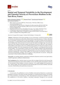
R E S U LT S Spatial and temporal variability in Gloeotrichia recruitment Variability within a year Recruitment of Gloeotrichia from the shallow sediments into the water column was highly variable in space and time (Fig. 2). Daily recruitment rates were often very low, with late-season pulses in most years (Fig. 2). The maximum daily recruitment rate varied >2 orders of magnitude among years, from lows of ∼600 colonies m–2 d–1 in 2011 and 2012 to >10,000 colonies m–2 d–1 in 2005, 2007, and 2010 (Fig. 2). Daily recruitment rates tended to be higher and more variable among years at Herrick Cove South (red lines in Fig. 2) and Newbury (blue lines in Fig. 2) than at North Sunapee Harbor and South of the Fells. In most summers, the pulses of recruitment occurred synchronously among multiple traps (Fig. 2), but the degree of synchrony varied among years and with the distance between traps (Fig. 3, Table 1). Daily recruitment rates generally peaked after doy 230 (18 August). Earlyseason peaks in Gloeotrichia recruitment occurred in the 2 y with the latest ice-out dates, 2007 and 2008 (Fig. 2), which led to a tendency for the peak daily recruitment rate to occur later when the ice went out early (ρ = –0.74). The late-summer peak occurred earlier in 2008 and 2010 (between doy 230 and 245) than in most other years (after doy 245). Temporal coherence among traps within a site was most striking in 2010, when recruitment to all traps at Newbury peaked 1 wk before recruitment to 3 of the traps at Herrick Cove South (Fig. 2). Recruitment dynamics were least coherent in 2008, when negative correlations between sites (Fig. 3) arose from strongly asynchronous fluctuations in recruitment (Fig. 2). Overall, D traps (those at different sites) tended to be least coherent and C traps (those at the same crates) tended to be most coherent, as evidenced by an increasing pattern moving from left to right within years in Fig. 3. In all years but 2012, the temporal coherence of traps differed among spatial scales (Table 1). Mean coherence of S traps did not differ (i.e., the crate from which a trap hung did not matter), but mean correlations between S traps and D traps differed significantly in 2008, 2009, and 2011 (Table 1). Variability across years Integrated recruitment rates varied from >10 colonies m–2 d–1 at North Sunapee Harbor in 2012 to nearly 3000 colonies m–2 d–1 at Herrick Cove South during 2010 (Fig. 4). Mean log10(x)-transformed integrated recruitment rates depended strongly on site, year, and their interaction (2-way ANOVA, year: F5,72= 58.8, site: F3,72= 133.1, year × site: F15,72= 5.7; all p < 0.0001, R 2= 0.92). Some sites and years had very high integrated recruitment rates (e.g., Herrick Cove South and Newbury during 2007 and 2010; Fig. 4), whereas others had low
Figure 2. Daily recruitment of Gloeotrichia echinulata (colonies m–2 d–1) into funnel traps at multiple sites in Lake Sunapee, New Hampshire, USA, for summers 2005–2012. The vertical black lines indicate the period during which statistics were calculated (days of the year 173–265 [22 June–22 September in non-leap years]). Sites sampled only with a single trap in 2005 are indicated with solid black lines. Otherwise, colors denote traps at the same site within the lake and line types indicate traps on the crate at a site, such that the same color and same line type indicate traps on the same crate at the same site. Note different y-axes on each panel.
584
|
Variability in Gloeotrichia recruitment
C. C. Carey et al.
Figure 3. Outlier boxplots summarizing the pairwise temporal coherence (indicated by Spearman rank correlation) of Gloeotrichia echinulata recruitment into funnel traps deployed in Lake Sunapee, New Hampshire, USA, from 2007–2012. Boxplots drawn as described in Fig. 1. Coding indicates different sites within the lake (D), at the same site but different crates (S), and at the same crate within a site (C).
recruitment rates (e.g., North Sunapee Harbor in 2008, 2009, 2011, and 2012). Overall, the North Sunapee Harbor site tended to have the lowest integrated recruitment rates, whereas Herrick Cove South and Newbury had the highest (Fig. 4). In many sites, the integrated recruitment rates declined through time, reflecting in part the lower rates observed in 2011–2012 (Fig. 4). Drivers of interannual variability in recruitment Summarized at monthly to summer-long time scales, the focal abiotic drivers fluctuated during the period from 2005–
2012 (Fig. S3). Cumulative annual precipitation ranged from 862.7 mm in 2012 to 1424.8 mm in 2005. Tropical Storms Irene and Lee in late August and early September 2011 marked a high point in precipitation (Klug et al. 2012) relative to a general decline over the study period. In August, when Gloeotrichia recruitment was high (Fig. 2), minimum daily air temperatures (Q1) increased ∼3°C from 2005 to 2012 (Fig. S3). Mean water temperatures were ∼23°C in most years, but lower in 2008 (22.0°C) and higher in 2012 (24.3°C), whereas SDs declined from a high of 2°C in 2006 to a low of 0.8°C in 2012. Median
Table 1. Mean temporal coherence of Gloeotrichia echinulata recruitment at different spatial scales in each year from 2007–2012 in Lake Sunapee, New Hampshire, USA. The F-test for the null hypothesis of no difference among spatial scales is indicated by F (df = 2,117 for all years) and the p-value. When p < 0.05, we used Tukey’s Honestly Significant Difference (HSD) test to run multiple comparisons. ND = no difference detected, D = different sites, S = same site but different crate, C = same crate. Mean Spearman rank correlation
ANOVA
Year
Different sites
Same site
Same crate
F
p
Tukey’s HSD
R2
2007 2008 2009 2010 2011 2012
0.60 0.08 0.51 0.50 0.45 0.43
0.71 0.40 0.69 0.62 0.60 0.42
0.76 0.56 0.75 0.65 0.62 0.54
3.83 23.01 6.17 4.28 6.64 0.80
0.02