MARINE ECOLOGY PROGRESS SERIES Mar Ecol Prog Ser
Vol. 431: 243–254, 2011 doi: 10.3354/meps09167
Published June 9
Spatial and temporal variability of red grouper holes within Steamboat Lumps Marine Reserve, Gulf of Mexico Carrie C. Wall*, Brian T. Donahue, David F. Naar, David A. Mann College of Marine Science, University of South Florida, St. Petersburg, Florida 33701, USA
ABSTRACT: Red grouper Epinephelus morio act as ecosystem engineers by excavating depressions (or holes) in areas of flat sandy bottom, which provide suitable habitat for themselves and numerous other species. To understand the spatial extent of the holes, which serve as spawning habitat, and determine how that habitat changes, high-resolution multibeam sonar data were collected in overlapping areas in 2006 and 2009 within Steamboat Lumps Marine Reserve. This marine reserve was established in 2000 and is located in the eastern Gulf of Mexico. Vertical profiles of the holes visually identified from the multibeam data were extracted to characterize hole shape and determine changes in the height, width, and slope of each hole over time and space. Results from this analysis indicated an increase in hole density from 110 to 141 holes km–2 from 2006 to 2009, respectively, with 181 holes detected in 2006 and 231 holes detected in 2009. Height and slope also increased between 2006 and 2009. The shape changes present in the 151 holes identified in the same location between the 2 survey years suggest that while hole shape varies due to red grouper maintenance, holes are constructed and maintained over time. The communication network determined from calculating a 70 m limit to red grouper acoustic communication showed an increase in communication overlap from 2006 to 2009, with over 95% of holes located within 70 m of their nearest neighbor. The increase in number and density of holes from 2006 to 2009 demonstrates that multiyear habitat mapping using active acoustic sonar is an effective method to monitor the presence and extent of red grouper spawning populations. KEY WORDS: Red grouper · Epinephelus · Multibeam sonar · Marine reserves · Holes · Habitat engineer · Gulf of Mexico Resale or republication not permitted without written consent of the publisher
INTRODUCTION Like all grouper species, red grouper Epinephelus morio are slow-growing, late-maturing, relatively stationary, and long lived fish. Red grouper are protogynous hermaphrodites that change sex from female to male between 5 and 10 yr of age (Moe 1969, Jory & Iversen 1989, Heemstra & Randall 1993, Musick 1999, Coleman et al. 2000, Sadovy 2001). These life history characteristics should make them vulnerable to overexploitation, especially in the Gulf of Mexico where a sizeable fishery exists. However, red grouper may be relatively resilient to fishing pressure because this species forms small polygamous spawning groups dispersed over large areas, unlike the large spawning aggregations typical in other grouper species (Cole-
man et al. 1996). Still, red grouper have experienced a truncated age structure and are currently considered Near Threatened by the International Union for Conservation of Nature (IUCN) (SEDAR 2009, Coleman & Koenig 2010, IUCN 2010). Red grouper spawn offshore (~70 m depth) during the late winter to early spring for ~4 mo, with peaks in April and May (Jory & Iversen 1989, Koenig et al. 2000). During this time, females approach males, which exhibit high site fidelity to an area of the seabed known as their ‘home territories’ (Coleman et al. 2010). If a male then successfully courts a female, they ascend up into the water column to spawn. Such offshore spawning habitat is likely to experience increased human disturbances as intense fishing in shallow areas drives fish population sizes down and
*Email:
[email protected]
© Inter-Research 2011 · www.int-res.com
244
Mar Ecol Prog Ser 431: 243–254, 2011
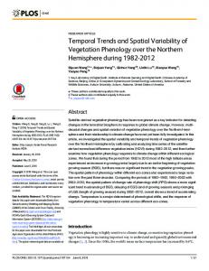
fisheries move offshore (Koslow et al. 2000, Coleman & Koenig 2010). Thus, locating both mature fish populations and spawning habitats essential to population stability are critical considerations for fisheries management (Coleman et al. 1996, Crowder et al. 2000). To alleviate fishing pressure on grouper aggregations during spawning, 2 marine reserves covering 200 n miles2 were established in June 2000 on the shelf break (50– 120 m deep) of the northeastern Gulf of Mexico (Fig. 1): Madison Swanson (29° 06’ N to 29° 17’ N, 85° 38’ W to 85° 50’ W) and Steamboat Lumps (28° 03’ N to 28° 14’ N, 84° 37’ W to 84° 48’ W) Marine Reserves (Coleman et al. 2004). Two important red grouper behaviors have been documented recently in these marine reserves: (1) sediment excavation (Scanlon et al. 2005, Coleman et al. 2010) and (2) sound production (Montie et al. 2011). In the present study, we focused on sediment excavation in Steamboat Lumps Marine Reserve and the potential for the 2-dimensional spacing of the holes to be within the known acoustic communication range of red grouper. In continental shelf areas with a sedimentary bottom, red grouper excavate large (5 to 25 m diameter) depressions (or holes) that they use as home territories (Scanlon et al. 2005). Red grouper excavate by carrying mouthfuls of sediment from within a depression to a short distance away and then depositing the sediment by flushing it through their opercles (Scanlon et
al. 2005, Coleman et al. 2010). In Steamboat Lumps Marine Reserve, holes are mainly observed to be dug and maintained by males who use this habitat as their home territory where they will spawn. Further inshore, juvenile (female) red grouper also exhibit this behavior (Coleman et al. 2010). Hole excavation is mainly found in areas where relief such as rock outcroppings is not present (Coleman et al. 2010). Excavation uncovers loose rocks such as cemented carbonate nodules, which provide an important source of substrate and refuge for organisms in areas where it was not previously available (Scanlon et al. 2005). Habitat preferences based on substrate composition influence the distribution of many marine organisms, especially benthic species (Day et al. 1989, Coleman & Koenig 2010). Additionally, the probability of observing other species is higher at holes where red grouper are present (active sites) compared to those where red grouper are not present (inactive sites) (Coleman et al. 2010). Holes can be observed using high-resolution acoustic sonar (e.g. side-scan or multibeam sonar) (Scanlon et al. 2005, Allee et al. in press; Fig. 2). In addition, the swim bladder in fish, including red grouper, can be detected with sonar because acoustic reflections result from the difference in density of the gasfilled swim bladder and the surrounding seawater (Misund 1997). Therefore, the application of active acoustic technology can provide high-resolution information on changes in bathymetry, including holes, and the presence of fish. The goals of this project were to study the distribution and dynamics of red grouper holes using 2 multibeam sonar surveys conducted 3 yr apart. Additionally, we aimed to quantify the percentage of holes potentially occupied by red grouper and estimate grouper acoustic communication ranges as a means to indicate marine reserve success and understand the groupers’ social system.
MATERIALS AND METHODS
Fig. 1. Madison-Swanson and Steamboat Lumps Marine Reserves located in the eastern Gulf of Mexico. Inset: 2006 and 2009 multibeam data overlapped in the hatched square within Steamboat Lumps Marine Reserve (black box)
Study area. The West Florida Shelf (WFS) extends over 200 miles from the Florida coast between the Florida Keys and the Mississippi River delta, creating a wide, gently sloping shelf. The inner WFS consists of a nearly flat, drowned and partially dissolved lithified carbonate (karst) platform covered by a thin layer of carbonate-siliciclastic sediment (Hine 1997, Brooks et al. 2003b). Five Holocene facies, or sediment veneers, have been identified overlying the bedrock of the central WFS: organic-rich mud, muddy sand, shelly sand, mixed siliciclastic/carbonate, and fine quartz sand (Edwards et al. 2003, Robbins et al. 2008). The distribution of each sediment type is highly varied along the
Wall et al.: Variability of red grouper habitat
inner central WFS and reflects both low accumulation rates and the lack of a single dominating source, all of which come from within or along the perimeter of the catchment (Brooks et al. 2003a). Scarped hard bottom systems are the only natural relief (< 4 m) (Obrochta et al. 2003). The lack of active coral reefs in this region is attributed to the effects of the high-nutrient, low-salinity Mississippi River discharge entrained in the Loop Current (Hallock 1988, Gilbert et al. 1996). Detailed descriptions of the WFS geology are provided in Randazzo & Jones (1997) and Jarrett (2003). Bathymetry mapping. Red grouper spawning habitat was mapped using a Kongsberg EM3000 multibeam swath sonar. The EM3000 operates at 300 kHz with 127 overlapping beams. Beam width is 1.5 × 1.5° with beam spacing of 0.9°, producing a 130 m swath transverse to ship heading. The vertical uncertainty of the EM3000 in a water depth of 100 m is 10 cm RMS with a 20 cm accuracy and 1 m positioning accuracy using an Applanix POSMV 320 system upgraded to a L1/L2 band that provides 0.02° RMS roll, pitch, and heading accuracy. Heave accuracy is 5 cm or 5% of the heave amplitude. Tide data were used to normalize sea level to a mean low low water (MLLW) chart datum. Multibeam data were collected in overlapping portions of Steamboat Lumps Marine Reserve on 27 July 2006 and 23 April 2009 (Fig. 1). The survey tracks were retraced to replicate the data collection process (Fig. 2). The specific site chosen here corresponded to the study site of another project that focused on passive acoustic monitoring of red grouper sound production. Therefore, this site was a location of opportunity where, from previous work, red grouper were known to be present. Due to the high cost of ship time and the lack of funding, only one small portion of the reserve was monitored as a pilot study. While analysis of multiple areas in Steamboat Lumps over time would have allowed for the detection of red grouper habitat usage throughout the reserve, we were not capable of such a study chosen for this pilot proofof-concept program. The multibeam data were displayed and calibrated using CARIS HIPS and SIPS 7.0 software. Corrections for roll, pitch, heave, and tide were applied. Since tide data were not available for 2009, a static offset of 0.53 m, which
245
was the mean difference between the 2 data sets at 100 randomly selected locations, was applied to allow direct comparison to the 2006 data. The short survey period, 103 min, allowed the offset to be static and did not need to account for any significant tidal ebb or flow (see ‘Hole profiles’ for further details). Depth thresholds were applied to remove data that were out of the range of depths encountered during the survey. Data were further filtered using a threshold of 3 standard deviations away from the moving mean depth. A vertical exaggeration of 5 and sun angle of 45° were applied to visualize the bathymetric features (Fig. 2). Hole profiles. Two-dimensional vertical profiles of data points that crossed each hole visually identified from the multibeam data were extracted for both years. The profiles best represent the characteristics of the hole including the deepest point (Fig. 3). These data were used to determine the location (latitude and longitude), depth (distance from the tide-corrected surface to the bottom of the hole), height (vertical distance
Fig. 2. Multibeam bathymetry data collected in the Steamboat Lumps Marine Reserve in 2006 and 2009. (a) 2009 multibeam data overlaid with the vessel tracklines of 2006 (dotted white lines) and 2009 (black lines). (b) 2006 multibeam data overlaid with red grouper holes detected in 2006 (d, N = 181) and 2009 (s, N = 231). White box: area where 2006 and 2009 hole profiles were extracted. Black box: see (c). (c) Magnified image of area in black box that illustrates the holes located in the multibeam data. Latitudinal bands are artifacts of the sonar swath overlap. Latitude and longitude are not shown to preserve the marine reserve
246
Mar Ecol Prog Ser 431: 243–254, 2011
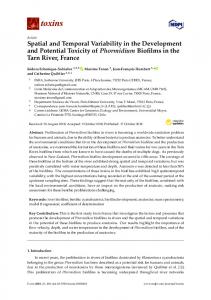
Fig. 3. Example hole profile created from data points (d) showing the shape characteristics that were measured (grey lines). Data points represent individual pulses of high-frequency sound (pings) from the multibeam sonar, from which measurements of depth (d), the distance from tide-corrected surface to hole bottom, height (h), the distance from the top of the hole to the bottom of the hole, and width (w) were made. (Q) Data point suspected to be caused by fish presence. Note the exaggeration in the vertical scale
from the depth of the hole edge to the depth of the hole center), width (distance across the hole), and slope (height divided by half the width) of each hole. The above-hole depth (hole height plus hole bottom depth) was calculated to determine an offset in the depth calibration between the 2 data sets. Although the static offset applied to the 2009 data greatly improved its alignment with the 2006 data set, any error in the actual absolute depth measurement will not affect the hole characteristics that were measured (height, slope and width) as they were determined by the difference of very precise (not necessarily accurate) depth measurements. For further discussion and analysis of this type of approach, see Wolfson et al. (2007). Due to differences in survey geographic coverage between the 2 yr (e.g. data were collected further south in 2009 than in 2006), only profiles within overlapping data sets were used. Areas in the data where sonar swaths overlap interfere with an accurate representation of the bathymetry and inhibit proper detection and hole characterization. Therefore, only areas with adequate bathymetry data coverage were used to detect holes. To identify corresponding holes in 2006 and 2009, holes detected in 2006 that were within 10 m of those detected in 2009 were assumed to be potentially the same hole and were inspected visually. As a conservative estimate, 10 m was chosen and encompassed the vast majority of holes coinciding between the years.
This analysis was completed using ESRI (Environmental Systems Research Institute) ArcGIS 10 software and was used to account for any georeferencing inconsistencies between the 2 data sets. The height, width, and slope of these holes were compared to determine changes in hole shape from 2006 and 2009. Significant changes in these parameters over the 3 yr period were tested using a paired t-test. Profiles were also analyzed to determine if a hole had been abandoned or was less defined (inactive) from 2006 to 2009, or if a hole had been created or was better defined (active) in 2009 compared to 2006. As the multibeam data consist of discrete data points (or pings), a 10-term polynomial was fitted to each hole profile to create a continuous cross-section. This analysis was done to mathematically characterize the general shape of the holes. Unfiltered (raw data) pings floating at least 10 cm above the seafloor along the hole profile were assumed to result from the presence of fish because they are distinct from the underlying seafloor (Fig. 3). To determine if a hole was active or inactive and to characterize the shape of active and inactive holes, we quantified the number of nonseafloor associated pings per profile and compared this count to the hole’s polynomial-derived shape and slope. The slope that characterized the steepness of the hole was calculated from each polynomial by subtracting the hole depth at 5 m to the left of the hole center (a placement always located within the hole) from the hole depth at the center and then dividing by 5 m (the horizontal distance from the hole depth to the hole center). We then determined if the hole slopes differed significantly as a result of height or number of nonseafloor associated pings. Hole distance and red grouper source level. The distance from the deepest point of each profile to the deepest point of the nearest profile was calculated in ArcGIS for 2006 and 2009. Histograms of between-hole distances for both years were created in MATLAB (Mathworks). Male red grouper produce sound during courtship and territorial behavior (Montie et al. 2011). To determine the potential communication network within the study area, the relationship between estimated grouper communication ranges and distances between the holes was analyzed. The intensity of sound produced by red grouper from 1 m away, also known as source level (SL), was assumed to be equal to the most intense received level recorded of a sound produced by a red grouper over many hours of recordings (Montie et al. 2011). Although red grouper are a benthic species and the substrate will interact with the propagation of sound, a cylindrical model (Urick 1983) is not practical due to the depth of the water column (~100 m) where red grouper produce sound without constraint from an air-water interface. Therefore, we
247
Wall et al.: Variability of red grouper habitat
applied a spherical spreading model as a conservative estimate of transmission loss (TLspherical): (1)
(2)
b
+
+
+
+ +
30
1
Width (m)
where R is range in m. With this model, we calculated the maximum acoustic communication range given SL and noise floor level (NL): R = 10(SL– NL)/20
a
35
Height (m)
TLspherical = –20 log(R)
1.5
0.5
+ + + +
25 20 15
where distance is in m and SL–NL represents the signal-to-noise ratio (SNR).
10
0
RESULTS Hole profiles
+
+
2006
2009
0.3
15
0.2 10 + +
0.1
5 0
0 +
+
2006
2009
Degrees (°)
+ +
Slope (m–1)
There were 219 profiles extracted from the 2006 data (1.88 km2 surveyed) and 278 profiles from the 2009 data (2.81 km2 surveyed). Thus, the grouper hole density over the areas surveyed was 116 holes km–2 in 2006 and 98 grouper holes km–2 in 2009. After restricting the study area to that which overlapped in the 2 data sets and removing profiles that were potentially undetectable in the other data set, there were 181 holes in 2006 and 231 holes in 2009, covering ~1.64 km2. These constraints resulted in a density of 110 and 141 grouper holes km–2, respectively. Height and slope of the holes increased significantly from 2006 to 2009 (Fig. 4). The 10 m buffer analysis found 151 profiles to be directly comparable between the 2 data sets. After comparing the height, width and slope of corresponding holes, only height and slope were significantly different over the 3 yr (Table 1, Fig. 5). Regression of the above-hole depth of the directly comparable 2006 and 2009 holes identified a close fit between the data sets (R2 = 0.9). Additionally, the mean of the absolute value of the residuals was 0.1 m. The number of new holes detected in 2009 was greater than the number abandoned after 2006 (Fig. 6). Out of 181 holes, 23 (13%) were identified in 2006 and not in 2009 (Fig. 7a,b). Conversely, 77 out of 231 holes (33%) were identified in 2009 and not in 2006 (Fig. 7c,d). There were 158 total non-seafloor associated pings found among the 23 inactive holes, which resulted in a median of 5 non-seafloor associated pings per hole (SD = 6). In comparison, 473 total non-seafloor associated pings were recorded among the 77 active holes, which equated to a median of 6 non-seafloor associated pings per hole (SD = 4). The mean of the hole polynomials calculated for each year showed an overall increase in the height and slope of the hole from 2006 to 2009 (Fig. 8a). However, the shape of the polynomials was variable (Fig. 8b). To
2006
+ + +
c
+ + +
5
2009
Fig. 4. (a) Height, (b) width and (c) slope for the 2006 (N = 181) and 2009 (N = 231) hole profiles. The central mark is the median, the box boundaries are the 25th and 75th percentiles, the whiskers extend to the 95th percentile and the outliers are plotted individually. With 95% confidence, medians were significantly different if the notch intervals did not overlap
Table 1. Shape parameters for holes (mean ± SD, N = 151) directly comparable between 2006 and 2009 surveys and results of the paired t-test analysis
2006 2009 p
Height (m)
Width (m)
Slope (m–1)
0.6 ± 0.2 0.7 ± 0.2 < 0.001
16.4 ± 3.7 16.3 ± 3.7 0.8
0.07 ± 0.04 0.09 ± 0.04 < 0.001
reduce this variability, the polynomials were separated into 3 categories of height: < 0.35, 0.35–0.70 and > 0.70 m (Fig. 9a,b) and 4 categories of non-seafloor associated pings: 0, 1–9, 10–19, and 20–29 pings (Fig. 9c,d). The mean polynomial of each group was calculated. Holes with greater height had a steeper slope. However, hole shape did not appear to be correlated with the number of non-seafloor associated pings, which was a proxy for potential fish presence. Linear regression of the slope and height for 2006 and 2009 showed a positive correlation and relatively good fit (Fig. 10a,b). The regression of slope and number of non-seafloor associated pings had a poor fit and low correlation (Fig. 10d). Over 90% of the profiles for
248
Mar Ecol Prog Ser 431: 243–254, 2011
Fig. 6. Multibeam data collected in 2009 overlaid with inactive holes that were filled in (d, N = 23) or active holes that were new or deeper (s, N = 77) between the 2006 and 2009 surveys
those corresponding to holes with at least 1 nonseafloor associated ping (potentially active holes).
Hole distance and red grouper source level
Fig. 5. (a) Height, (b) width and (c) slope for holes that corresponded across the 2006 and 2009 surveys (N = 151). The black line shows a 1:1 ratio. Data points above this line indicate an increase in that parameter from 2006 to 2009
2006 (164 out of 181) and 2009 (214 out of 231) contained at least 1 non-seafloor associated ping. Slopes corresponding to holes with 0 non-seafloor associated pings (potentially inactive holes) did not differ from
The sound pressure level (SPL) thresholds of red grouper hearing within the frequency range of red grouper sound production (100 to 300 Hz) are estimated to be 100 dB re 1 µPa based on hearing thresholds of gag grouper Myceteroperca microlepis (S. Larsen & D. A. Mann unpubl. data). Therefore, with a median NL of 105 dB re 1 µPa, the noise floor, rather than hearing thresholds, will limit communication distances. With an estimated SL of 142 dB re 1 µPa (Montie et al. 2011), sound produced by one red grouper is
Wall et al.: Variability of red grouper habitat
249
Fig. 7. Example changes in quality of holes (black circle) observed in multibeam data between the 2 surveys. Same hole detected in (a) 2006 and (b) 2009 that became less well-defined and a second hole detected in (c) 2006 and (d) 2009 that became more well-defined
Fig. 8. (a) Mean hole height and (b) standard error by year visualized with a 10-term polynomial applied to each hole profile. Note the exaggeration in the vertical scale
250
Mar Ecol Prog Ser 431: 243–254, 2011
Fig. 9. Mean polynominal shape of hole profiles grouped by (a,b) maximum hole height for (a) 2006 and (b) 2009 and (c,d) non-seafloor associated pings for (c) 2006 and (d) 2009. Note the exaggeration in the vertical scale
Fig. 10. Linear regression (black line) and fit statistic (R2) for mean slope and (a,b) mean height of holes measured in (a) 2006 and (b) 2009 and (c,d) mean slope and number of non-seafloor associated pings, which indicate relative fish abundance, for holes measured in (c) 2006 and (d) 2009
251
Wall et al.: Variability of red grouper habitat
Fig. 11. Nearest neighbor distance (m) between holes detected in (a) 2006 (N = 181) and (b) 2009 (N = 231). Note the difference in greyscale bar
calculated to be detectable by another red grouper up to 70 m away. Due to the short transmission distance and low acoustic frequency, acoustic attenuation due to absorption is negligible. Maps of the distance estimated between the deepest point of the hole profiles in 2006 and 2009 showed that the holes cluster towards the center of the study area (Fig. 11). The effective acoustic communication network between holes, based on the maximum range estimate of 70 m, is illustrated in Fig. 12. Histograms of the betweenhole distances show over 95% of holes are located within 70 m of their nearest neighbor (Fig. 13). The median distance between nearest holes is 26 m (SD = 15) and 24 m (SD = 28) for 2006 and 2009, respectively.
DISCUSSION High-resolution multibeam bathymetry data collected in 2006 and 2009 in Steamboat Lumps Marine Reserve allowed detailed documentation and characterization of holes excavated by red grouper. Analysis of these data showed a significant increase in number, height and slope of holes over this 3 yr period. Direct comparisons of holes detected in both 2006 and 2009 indicated significant changes in height and slope. The changes in these parameters suggest that hole shape could Fig. 12. Red grouper communication network showing the estimated maximum vary because of maintenance by red estimated ranges of grouper acoustic signals (white circles), which are estimated groupers and that holes are conto be 70 m away from grouper holes located in (a) 2006 and (b) 2009. Distances structed and maintained over time > 70 m (black) were suspected to be outside of the effective communication range of red grouper (Coleman et al. 2010). Low sediment accumulation rates in the Gulf of Mexico also prevent quick infill and shape modification of holes in the absence of red grouper (Brooks et al. 2003a). Active vents are generally steeper and deeper than inactive vents indicating that increased height in conjunction with slopes greater than the angle of sediment
Fig. 13. Number of pairs of red grouper holes found at different nearest neighbor distances between holes identified in 2006 (black) and 2009 (gray) and binned into 20 m intervals. Over 95% of the holes in both years were within 70 m of their nearest neighbor and therefore likely contained individual fish within acoustic contact. Dashed line indicates maximum distance of red grouper communication
252
Mar Ecol Prog Ser 431: 243–254, 2011
repose might signify active hole occupation (Saleem 2007). Although overall hole slope increased significantly from 2006 to 2009, the lack of correlation between hole slope and number of non-seafloor associated pings suggests the shape does not change significantly if unoccupied unless bad pings are poor indicators of fish. Ground-truthed data are needed in concert with simultaneous multibeam data collection to determine if hole occupation can be established based solely on the presence of non-seafloor associated pings. Despite collecting bathymetry data in depths ranging from 69 to 81 m, the median depth for all holes was 71.2 m with a standard deviation of 0.6 m. The reason for the clustering of holes within this depth range is unknown. Initially, we suspected the clustering to be related to constraints of bottom composition preventing hole excavation since sediment type distribution is highly varied throughout the WFS (Brooks et al. 2003a). Yet, backscatter data, which is useful for identifying bottom type (Dartnell & Gardner 2004), collected concurrently with the bathymetry data indicated uniform sediment distribution in our study area. If more than just social behavior is at hand, additional factors such as water temperature, bottom currents and loop current intrusions may be influencing the location of red grouper holes in this area. Scanlon et al. (2005) calculated hole density in Steamboat Lumps to be 250 holes km–2 from side-scan sonar data collected in 2000, which is roughly double the hole densities measured with multibeam sonar in this study (110 and 141 holes km–2 in 2006 and 2009). The specific 0.4 km2 area that they surveyed may have not directly overlapped with the area surveyed in this study. In addition, the hole density calculated by Scanlon et al. (2005) focused on a subset of data that was heavily populated with holes and then extrapolated the density estimate throughout the study area. We calculated hole density over the entire survey area, which consisted of dense and sparse areas of holes. Scanlon et al. (2005) classified a grouper hole visually from the interpolated raster created from side-scan sonar data. By examining the multibeam data on the data point level, we were able to exclude artifacts and errant pings that appeared to be holes when solely examining the backscatter raster data. Although it aides visually, applying a vertical exaggeration to interpolated bathymetry maps can trick the eye into believing a hole exists when it is actually an artifact of the data. This density discrepancy could be compounded further by the differences in sonar technologies used. Interpreting the backscatter shadows in side-scan sonar data can be difficult due to the angular uncertainty, their dependence on the direction of the boat, and the varying grazing angles, which can change throughout a survey and across the survey track. The backscatter
shadows can be misleading because they can result from changes in seafloor geology or biology in addition to relative depth. With multibeam data, shadows can be created in software during post processing and will provide a consistent ‘grazing’ angle across the track regardless of depth. Side-scan sonar devices offer more refined backscatter data to determine bottom composition and provide higher resolutions when towed close to the bottom compared to hull-mounted multibeam ones. The increase in number of holes detected from 2006 to 2009 is consistent with increases in hole density and habitat usage, potentially the result of an increased grouper population. We attempted to identify if red grouper or other species were present within or near holes using non-seafloor associated pings. The percentage of potentially inactive holes (0 non-seafloor associated pings) decreased from 9% in 2006 to 5% in 2009, which also supports an increase in active holes. As fish very close to (