Spatial Clustering Algorithm Based on

Spatial Clustering Algorithm Based on Neighboring Structure Approach Arief F Huda, Ito Wasito, T. Basaruddin, Mujiono S

Spatial Clustering Algorithm Based on Neighboring Structure Approach 1

Arief F Huda, 2Ito Wasito, 3T. Basaruddin, 4Mujiono S, Mathematic Dept, UIN Sunan Gunung Djati Bandung, [email protected] 2, Computer Science, Universitas Indonesia,[email protected] 3, Computer Science, Universitas Indonesia, [email protected] 4, Informatic Dept, Universitas Mercu Buana,[email protected] 1,

Abstract Clustering of spatial data is applied on information of object description (non-spatial attributes) and an object location (spatial attributes). Based on the first law of Geographic’s, the spatial attributes have patterns in their neighboring relationships. The patterns of neighboring relationship are found by clustering method that is proposed in present research. The clustering method is applied on non-spatial attributes which is represented as a non-numerical form and spatial attributes which is represented as sequence form simultaneously. The sequences represent the pattern of data linkages to its environments i.e. the specific data with its neighbors which are located in north, east, south and west direction (stated as a particle).The particle’s element is composed as sequences where each sequence consists of nine elements counted from the first element to ninth element. The particles are grouped based on the similarity of their constructor elements. Similarity of particles Pi, Pj is measured based on 9

sim( Pi , Pj )   S ( pik , p jk ) with S(pik, pjk) = 1 if pik = pjk and S(pik, pjk) =0 if pik  pjk. Two particles k 1

are defined as similar if their similarity value is greater than a certain threshold value. The experiments of the proposed method have been implemented on the simulated and various real applications data. Overall, the experiments show that the performance of the proposed method has promising results such that clusters based on neighbor structure could approximate arbitrary shape of object very well. Keywords: Spatial Clustering, Raster Data, Non-numeric, Sequence, Neighboring Structure

1.

Introduction

The rapid growth of data collections provides us with a great number of data, making manual analysis more difficult to conduct. The majority of the data consist of spatial elements. Furthermore, the need to analyze the data increases as the number of available data keeps growing, most of which contains location (spatial) elements [1]. The rapid growing applications of spatial data cover the following fields: (1) cellular communication data, (2) internet data, (3) Global Positioning System (GPS) utilization data, (4) weather data, and (5) population migration data. Two attributes of a spatial datum are object description (referred to as non-spatial attribute) and information related to spatial elements (referred to as spatial attribute). Both of them are essential components of a spatial datum. The spatial information represents the relative position of one object datum compared to another, the relative position of an object datum in a particular observation area, or both types of positions. The other implication is that the relative position also reveals the function of a spatial linkage. Such linkages can be defined in terms of their distance, neighboring object data, gradient, or certain system configurations [2][3]. Clustering is one of data analytical methods which work in an unsupervised environment. Clustering method divides data into some groups (clusters) without any prior knowledge. Those groups can be meaningful, useful, or both. To achieve this goal, the clustering process has to be able to recognize the natural structure of data [4][5][6][7]. A process of spatial clustering has to include spatial elements of the data. Without those spatial elements, this process cannot be regarded as a spatial clustering process [8]. Unfortunately, spatial attributes are often implicit in a spatial dataset [9]. Recently, many spatial clustering algorithms have been developed for spatial datasets. Although the method of clustering can effectively accommodate spatial attributes, we cannot simultaneously process non-spatial attributes together with their spatial

Journal of Convergence Information Technology(JCIT) Volume8, Number16, November 2013

25


counterparts [10]. In this research, we propose a novel clustering algorithm that is capable of processing both spatial and non-spatial attributes simultaneously by using the neighboring structures of the spatial data presented in a raster format. Non-spatial attributes are presented in pixel values of a raster data. Some of clustering algorithms are extended to spatial clustering algorithms by applying spatial attributes[1],[11]. To handle spatial attributes, some algorithms use spatial indices, such as k-d tree, Rtree, and Delaunay triangulation [9],[10]. Developing these indices takes time and requires space computation not less than O(n log n) [12]. The method developed in this research is based on a raster spatial dataset, so there is no need to develop any spatial index. This clustering method results in patterns which take the form of irregular shapes clusters. These patterns are obtained from the neighboring structures of data elements. Since structure with similar elements has been identified as having similar patterns, the patterns in adjacent locations must also form irregular shapes. This method can be used to cluster spatial data which are available in picture formats, such as pictures taken by satellite and MRI, as well as pictures taken by a camera or a video which is called SCANS (Spatial Clustering Algorithm Based on Neighboring Structure).

2.

Related Works

The process of clustering algorithms can be categorized into two types: (1) the process of clustering execution and (2) the model of the data being used. A more general categorization consists of hierarchical clustering, partition clustering, density clustering, and grid clustering [1], [6], [13]. Some clustering algorithms of spatial data are the results of an extension from previous clustering algorithms [1],[14]. Therefore, the categorization of spatial data clustering algorithms follows the categorization of common clustering algorithms. The conversion of common clustering algorithms into spatial clustering algorithms is done by involving spatial elements in the clustering algorithms. Each clustering algorithm has its own unique way of involving spatial elements. The following paragraph presents some spatial clustering algorithms which are the extensions of usual clustering algorithms. Partition method divides data into subsets or partitions by evaluating the distance between data and cluster representation. Some proposed and developed algorithms which are based on partition method are k-means, k-medoid, fuzzy k-means, PAM, CLARA, and CLARANS [15], [16], [17]. CLARANS algorithm enhances PAM and CLARA algorithms in terms of their computation efficiency. Two methods of clustering which adopt CLARANS algorithm for spatial data are termed spatial dominant or SD approach (CLARANS) and non-spatial dominant or NSD approach (CLARANS) [16], [18]. CLARANS algorithm has also been implemented for spatial data in the form of Raymond’s polygon [16]. Some algorithms that perform clustering process based on density are DBSCAN, DENCLUE, and OPTICS [6], [19]. Sander extended DBSCAN by involving spatial elements and non-spatial elements simultaneously to cluster spatial data in 2 to 5 dimensional format [20]. DBCLASD is another extension of DBSCAN in spatial clustering algorithm [6]. Likewise, the density-based clustering algorithm developed by Yang et.al. (2010) and Liu et.al. (2012) was extended by using Delaunay triangulation [9], [10]. Using a spatial index such as Delaunay triangulation takes more time for computation. Therefore, to reduce the time needed for this process, the research used raster format for representing spatial datasets. There is another kind of clustering algorithm method that can be performed on non-numerical data. Some non-numerical data are presented in sequence, so clustering algorithm is based on that format. Studies on clustering method for sequence format have been conducted [21], [22] and applied on spatiotemporal brewery and crime data [23]. Kakkar used Generalized Suffix Tree (GST) approach to cluster temporal data in sequence format. The results of a temporal pattern are then clustered on the basis of its location (space) by applying Euclidean distance measurement [23]. Kakkar clustered spatial attributes by using Euclidean distance, so it cannot perform any other spatial property, such as adjacent or neighboring data objects. In this study, the neighboring structures are presented in sequence format and then clustered based on the sequence.

26


3.

Spatiall Clusteringg Based On n Neighboriing Structu ure (SCANS S)

Inn a spatial poiint of view, eaach data objecct contains som me surroundinng data. This ddata object andd its surrroundings devvelop three kinnds of relatioonships: distannce, directionn, and topologgy. Waldo Toobler (19770) stated thatt the first Law of Geographiic is that “Everrything is relaated to everythhing else, but nnear thinggs are more related r than ddistant things”” [24]. Based on this law, certain objectts have a stronnger relattionship to clloser objects tthan to other farther objeccts. The varieety of these reelationships iss an interresting topic in the field oof spatial dataa exploration. Therefore, thhis study propposes a clusteering methhod which is developed onn the basis off the variationn of data direcction relationsship structure and calleed Spatial Cluustering based on Neighborinng Structures (SCANS). M Moreover, in tthis study we ppropose similaarity parameteer that is based on the neighhboring structtures of a data object. T These neighboring structuress are developeed by certain objects o due to their adjacenccy in a diirectional relaationship. Thee degree of similarity s of neighboring structures is used to evalluate simiilarity measuree.

3.1.. Properties of Spatial D Data A spatial data element contaains informatioon about the shhape, dimensiion, and/or loccation of an obbject relattive to a speciific area. Theree are some typpes of spatial eelement, such as point patteern data, field data, areaa data, and spatial interactioon data [25]. Spatial interaaction data is a relationshipp (pairing) patttern amoong data in a pparticular locattion. The dataa used in this sstudy take the form of spatiaal interaction. The interractions amonng the mares arre defined on the basis of neeighboring pattterns in a partticular area.

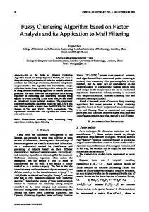
Figure 1: S Spatial data inn raster form S Spatial data contains linkagge characterisstics based onn its relative position to otther data objeects. These linkage chaaracteristics arre based on thhree aspects: ddistance, directtion, or topoloogy. The distanncebaseed linkage is tthe comparisoon between ann object’s disttance value annd others’. Thhe direction-baased linkage representss the relative pposition (in direction) of onne object with respect to othher objects. Laastly, the ttopology-baseed linkage reppresents a partticular relationnship which reemains unchannged even thoough two or more neiighboring objects have beeen given som me treatments,, such as rottation, scalingg, or translation. Includding in this toppological relattionship are “ddisjoint”, “meeet”, “overlaps””, etc. [1], [266].

Figurre 2: Ddirectioon relationshipp based on thee compass direection point off view D Direction-base ed relationshipp generally usees directional measurementt. An object iss assumed to hhave a dirrectional relattionship with rrespect to otheer objects locaated in the norrth, south, wesst, east, north east, e

27


north west, south east, and southwest. This study uses the variation of these directions as a basis for cluster determination method.

3.2. Terminology An object is surrounded by some neighboring objects which are given labels based on their relative directions to the object (see Figure 2). A neighboring structure is composed of one object and other surrounding objects. The observation utilizes this group of objects; this group is referred to in this paper as a “particle”. A cluster is defined as a group of particles with a fixed degree of similarity. The similarity degree is similarity among the sequences. It is used because the particles are in the form of a sequence. Some other technical terms used in this method are sequence, subsequence, particle, nucleus, candidate, and core. Below are the definitions. Sequence and subsequence Sequence is a collection of data which is composed sequentially. The position (order) of data is essential in a sequence. A sequence is formally defined as follows. Definition 1: Let T = {T1, T2, ..., Tm} be a set of pixels. A sequence, S, is S = , where siT In this study, data are composed in sequence form, and their patterns are defined on the basis of the similarity among some subsequences.

A subsequence is defined as follows: Definition 2: Let T = {T1, T2, ..., Tm} be a set of pixels. A sequence, Q, Q = is the subsequence of S, with S = , if  1≤ j ≤ m-1, ij < ij+1 and  1 = 

(2) (3)

Pi, Pk are the pparticles that make up the ith and kth canndidate. The tthreshold can be determineed in accoordance with tthe conditionss of the data annd the desiredd cluster. Therre is no rule too choosing onne of two equations. Thhe core describbed in figure 9 used the equaation 2. F Figure 9 is an illustration off the main corres obtained. T To simply com mpute this subbsequence, Divvide and Conquer algoorithms [28] caan be employeed.

31


Figure 88: Pattern or m main core T componennts recorded inn the core are subsequence and constitueent particles. B The By identifyingg the posiition of the paarticle we can visualize the particles as illlustrated in fiigure 10. In geeneral, the cluuster can be obtained byy 2-dimensionnal field, as illlustrated below w.

Figuree 9: Cluster thaat formed from m pattern of paarticles o the cluster ccan be used too see Inn addition to sspatial patternn formation in the form fieldds, the results of the co-occurrencee of an object. Suppose tthe core is a subsequencee {-kja-kbb-},, the informaation obtaained by it is nnucleus, and arround nucleuss there are k (nnorth), j (northh-east), k (east), b (south-west), b (south). As for the sign '-', m meaning for evvery particle hhas a subsequeence which thhey will be, inn the posiition '-' differeent constituentt elements. If tthere are 100 pparticles with the subsequennce, the objectt can be sseen as a scenne, surroundedd by objects k,, j, b (with thee direction annd number of eeach as explained earliier) there are 1100 events.

5.

Experiimental Evaaluation

T developedd method has been tested bby using simulated data andd real data. Thhe simulated data The weree made four tyypes that repreesent several ttypes of shapee such as rectaangular, circulaar and bent cuurve. Whiile real data ussed are brain image, biologiical tissue and batik motif. T image datta consists of several pixel represented inn a 2 dimensional matrix. T The The value of each e pixeel for grey im mage is a greyy scale value; meanwhile, ffor the color iimage, the pixxel values aree the valuue of red, greeen and blue sccale. The pressent study used grayscale im mage data. Thhe grayscale vvalue was transformed into non-num merical data. The T data, thenn, were clusteered with neigghboring struccture baseed spatial clusttering algorithhm. S Steps of the exxperiment are taken as folloows: preproceessing, clusterring, visualizinng and validatting. The preprocessingg is preparing data into clusstering algorithhm. Then clusstering algorithhm is done byy the methhod as propossed in this reesearch. The ppatterns of cluuster are visuualized into diifferent colorss for diffeerent clusters.. Visualizationn shows the siimilar neighbooring structure or cluster inn their location of imagge. Silhouette index is used to validate thhe strengthen of o resulting cluuster. is done to m P Preprocessing make data fit into the algoorithm. The fi first steps of ppreprocessingg are resizzing data intoo less than 2300x230 pixels. Afterwards, ddata are transfformed into tyype of image file,

32


suchh as black andd white, 16 bit color, and 2256 colors. N Next, the data are transform med into graysscale imagge and the lasst are transform med from pixxel value into non-numeric. The same inttervals are useed to transform numeriic value into nnon-numeric vvalues that aree making inteerval in 25 froom 0 to 255 ppixel valuues. S Silhouette indeex is one of clluster validations which usee dissimilarityy measuremennt of one datum m to anotther within its cluster and annother closest cluster. The vvalues are -1 – 1 meaning thhat they are biggger thann 0.7 (lableledd with a strong structure oof cluster); m more than 0.5 is labelled w with a reasonnable struccture of clusteer; more than 0.25 is considdered a weak structure of clluster. And the other valuess are conssidered non suubstantial struccture[15].

5.1.. Simulated D Data Sim mulated data iimages madee are as follow ws: 1. 2. 3. 4.

A simple spaatial pattern suuch as rectangular image (D Data set 1, figuure 11.a) A spatial patttern such as composite recctangular like the letter "n" and circular like the letter “o” (Data set 2, ffigure 11.b) A spatial patttern such as ccharacter   mutually entryy (Data set 3, figure 11.c) A spatial paattern such ass three bent ccurved lines, hhorizontal andd vertical straaight line andd the layered letter O (Data set 4, figure 11.dd)

F Figure 10: Daata in several pattern p and vissualization off spatial clusterr T data size oof all simulateed data set are shown in tablle 2 and the im The mage shape arre shown in figgure 4. Tab ble 1: Threshoold (% of partiicles number) with their relaated percentagge of clusteredd particle numb mber andd cluster numbber.

T Threshold usedd in this algorithm are minim mum elements of subsequennce and minim mum particles that form med one clusteer. The first tthreshold usedd 4 elements; it means the subsequence is different iff the

33


sam me elements off two or more subsequence are a less than 44. In the experriment for secoond thresholdd, we got threshold valuue as much aas 3-10% of aall data. The relationship between b clusteered particles and secoond threshold iis described inn figure 5.

Figure 11: Second thresshold and perccentage of clusstered data N Number of cluuster in data seet 1 for threshoold 1% is 13 aand for threshoold >=2% is 3.. While in dataa set 3, foor threshold 1% %, 2%, and >= =3% are 13, 5, and 3 respecctively. Patternns of cluster frrom data set 1 and 3 are shown below w,

T There are simiilar values of data d in data seets 1 and 3 so that the samee cluster are prroduced. The first clusster is the {kkkk kkk kkk}, w with the numbber of elementts is 9, the nuumber of particcles that makee up the cluster is 30331 for data seet 1, and 1383 for data sett 2. In data sset to 1 and 3 the patternss are rectaangular shapee (no arch bouundary). The fiirst cluster {kkkk kkk kkk} iis the backgroound of the im mage. The number of paarticles that maake up the struucture of existting {kkk kkk kkk} is 3031 for data set 1 and 13833 for data set 2. While clusster {000 000 000} are recttangular shapee, and cluster {kkk -kk ---} is a part of the outskirrts of the clustter object boxx. The other paarticles are ouutlier that is upp to 0.5% for data set 1 and 4.3% forr data set 3. T previous condition alsso occurred inn data set 2 and 4, but thhere are archh boundaries. The The bounndaries make more patternss of cluster. T Therefore, if thhe second clusster is 3-10% then there aree 14 clussters in data seet 2 and 19 cllusters in dataa set 4. First aand second cluuster are backkground and bbody objeect of data, resspectively. Thee rest of patterrns are from boundary bodyy objects. Tab ble 2: Silhouettte validation of simulated ddata

5.2.. Real Data T method has been testedd in some real data like hum This man brain imagge, biological ttissue, and battik’s motif. The real sspatial data arre more compplicated than simulated daata, so they will w produce more m

34


clussters and high value of outliier. The visuaalization of cluustered patternns is top 9 ressulting clusterss (in particles element)).

Figure 12: Hum man brain imaage and visualiization of braiin image clusteer man Brain Im mage Hum H Human brain images have been clustereed spatially byy this methodd. In the previious analysis,, the clussters are formeed if the num mber of constittuent articles is above the threshold, theen for the sakke of otheers, it can bee analyzed byy members off the smaller number of clusters c (outliiers). Afterwaards, com mparison amonng the data andd other data, rresulted whethher there are ddifferences in ccluster-forminng or not. It is useful tto detect outliier in data sett, like “cancer cell” since this phenomeenon is smalleer in num mber than norm mal cells. In thhis case, only significant clusters are disccussed. Brain images testedd are the brain images that are availlable at http:///brainmaps.orrg. We selecteed Homo sapiiens brain imaages mber 300, 380,, 420 and 660 applied to thiis algorithm. S Size of brain iimage data is an about 200xx150 num pixeel size, the parrticles obtainedd are about moore than 5500 particle, and nnumber of cluuster are 601-11041. The number of daata that clusterred are > 72% (outlier < 28% %), it mean 722% particle aree forming clussters and they have pattterns. Result of clusteered particle oof data set of bbrain image Table 3: R

F Figure 13 illusstrates the braiin image (figuure 13. a, b, c, d) and the visualization of cclusters (figure 13. a, b,, c, d). They vvisualize top 9 clustered pattterns that havee the greatest nnumber of connstituent particcles. Table 3 visualizess the image siize, numbers oof formed partticles, numberr of clustered particles, num mber of cllusters and thrreshold. Silhouuette index shhows the strongg cluster of alll data set in brrain image.

35


Biollogical tissue imaging Inn addition to bbrain images, biological tisssue images arre analyzed byy this method.. This methodd can form m clusters of sstructure of thhe groups thatt exist in bioloogical tissue iimages. The ffirst image (figgure at 14.aa) is image frrom [27],, and the restt are available www w.udel.edu/bioology/Wags/hhistopage/colorrpage/cb/cb.httml.

Figure 13: Biologiccal tissue and ccluster visualiization F Figure 14 illuustrates the biiological tissuues clustered by this method (figure 144. a, b, c, d) and visuualizes their cllusters (figure 14. e, f, g, h)). Compared w with the result of the brain iimage (figure 13), the visualization of biologicall tissues did nnot show goood clusters. B But table 4 shhows that > 83% 8 particles have beeen clustered (eexcept data sett 1 and 3 are > 48.7%) sincee cluster mem mbers are unevenly spreead. Silhouettee index show ws that data seet 1 and 3 haas strong clussters, but dataa set 2 and 4 are reassonable clusterrs. Table 4: Result of clusstered data of bbiological tisssue image

Batiik’s pattern A Another appliccation is imagge of “batik” motif. Batik’ss motif is a ppattern on the fabric used ffor a variety of needs, for example clothing. c Batikk is a fabric paattern used to outfit a worldd cultural heriitage of IIndonesian country. Motif is numerous and varied, eeach of whichh shows certaain character, and reprresents the origgin of the mottif region. Witth this algorithhm, several maajor motif pattterns can be foound. The main motif ppattern can be used to distinnguish one mootif to anotherr. This methodd was executeed to obtaain cluster 4 (ffour) batik’s motif. m

36


Figure 14: Onne of batik’s ppattern and vissualization of spatial s cluster.. F Figure 15 illusstrates batik m motif image (ffigure 15. a, bb, c, d) and viisualization off clustering reesult (figuure 15. e, f, gg, h). The visualization off result of cluusters shows tthat there aree a good clusters, perccentage of clusstered particlee are > 94% (ttable 5) since the top 9 clussters have mucch more mem mbers thann the others. Inn other word, the cluster meembers are noot evenly spreaad. Silhouettee index shows that stronng cluster onlyy for data set 4, 4 and the otheers are reasonaable cluster. Table 55: Result of cluustered particlles from batik data set

6.

Conclu usion and F Future Work

T proposed clustering m The method uses nnon-spatial atttribute and sppatial attributee simultaneouusly. Spattial attribute is position of ppixel in rasterr data. The noon-spatial attribbute is a pixel value or a vvalue objeect presented in the form of symbols (non-numeric) ( . The methodd is based onn the neighbooring struccture using diirectional relaationship. Thenn the algorithhm was emplooyed in the sequence clusteering methhod. C Clustering resuults that makee up a pattern formed an arrbitrary shape in a 2-dimennsional space. The patteerns that form m thick shape are a easy to visuualize. But paatterns of thin aarch-shaped oobject cannot fform clussters as well aas it is hard too visualize. Siilhouettes indeex of clusterinng results show ws the strengtthen clussters in simulaated and brainn data, but tissue and batikk’s motif data have not stroong cluster forr all theirr data sets. T co-occurreence and/or coo-location of data analysis can be carriedd out by usingg the neighbooring The strucctures of the adjacency and the informaation obtainedd from each ccluster. The nuumbers of cluuster weree large so thaat a further trreatment is reequired. This can be done by involving an expert to see wheether the clusteer needs to be merged with tthe existing cllusters or not.

7. [1] [2] [3]

Referen nces A. Varlaroo, “Spatial Cluustering of Strructured Objeccts,” Universitty of Bari, Itally, 2008. R. P. Haaining, R. Keerry, and M. A. Oliver, ““Geography , Spatial Dataa Analysis , and Geostatisttics : An Overrview,” Geogrraphical Analyysis, vol. 42, no. 1, pp. 7–31, 2010. H. Robertt, Spatial Dataa Analysis, Theory and Pracctice. Cambriddge Universityy Press, 2004.

37


[4] [5] [6] [7] [8] [9] [10] [11] [12] [13] [14] [15] [16] [17] [18] [19] [20] [21] [22] [23] [24] [25] [26] [27] [28]

K. Pang-Ning, Tan; Michael, Steinbach; Vipin, “Ch 8. Cluster Analysis :,” in in Introduction to Data Mining, 2006. B. Mirkin, Clustering for Data Mining A Data Recovery Approach. Chapman & Hall/CRC, 2005, pp. 1–278. Margaret H. Dumham, “Ch 8. Dunham Spatial Mining,” in in Data Mining, Introductory and Advanced Topics, New Jersey: Pearson Education, Inc., 2003, pp. 221–244. A. K. Jain, M. N. Murty, and P. J. Flynn, “Data Clustering: A Review,” ACM Computing Surveys, vol. 31, no. 3, pp. 264–323, 1999. S. Shekar and R. R. Vatcavai, “Spatial Data Mining Research by the Spatial Database Research Group, Univ of Minnesota.” X. Yang and W. Cui, “A Novel Spatial Clustering Algorithm Based on Delaunay Triangulation,” J. Software Engineering & Applications, vol. 2010, no. February, pp. 141–149, 2010. Q. Liu, M. Deng, Y. Shi, and J. Wang, “A Density-based Spatial Clustering Algorithm Considering Both Spatial Proximity and Attribute Similarity,” Computers and Geosciences, Elsevier, vol. 46, pp. 296–309, 2012. S. Chawla, S. Shekar, W. Wu, and U. Ozesmi, “Extending Data Mining for Spatial Applications: A Case Study in Predicting Nest Location.” F. H. Razafindrazaka and M. Sciences, “Delaunay Triangulation Algorithm and Application to Terrain,” no. May. pp. 1–32, 2009. E. Chandra, “A Survey on Clustering Algorithms for Data in Spatial Database Management Systems,” International Journal of Computer Applications, vol. 24, no. 9, pp. 19–26, 2011. S. Shekhar and S. Chawla, Spatial Databases A Tour. New Jersey: Prentice Hall, 2003, pp. 1– 284. L. Kaufman and P. J. Rousseeuw, Finding Groups in Data: An Introduction to Cluster Analysis. New Jersey: John Wiley & Sons, 1990, pp. 1–355. N. Raymond T. and J. Han, “CLARANS : A Method for Clustering Objects for Spatial Data Mining,” IEEE transactions on Knowledge and Data Engineering, vol. 14, no. 5, pp. 1003– 1016, 2002. Rama.B, Jayashree.P, and S. Jiwani, “A Survey on clustering,” International Journal on Computer Science and Engineering, vol. 02, no. 09, pp. 2976–2980, 2010. F. Zhou and S. K. Zhan, “Analysis of spatial clustering of disease,” Chinese journal of preventive medicine, vol. 28, no. 6, pp. 337–339, 1994. M. Ester, H. Kriegel, J. Sander, and X. Xu, “A Density-Based Algorithm for Discovering Clusters in Large Spatial Databases with Noise,” in 2nd International Conference on Knowledge Discovery and Data Mining (KDD-96), 1996. J. Sander, M. Ester, H. Kriegel, and X. Xu, “Density-Based Clustering in Spatial Databases : The Algorithm GDBSCAN and its Applications,” Journal Data Mining and Knowledge Discovery, vol. 2, no. 2, pp. 169 – 194, 1998. B. Dorohanceanu and C. Nevill-Manning, “A Practical Suffix-Tree Implementation for String Searches,” Dr. Dobb’s Journal, 2000. K. Fredriksson, G. Navarro, and E. Ukkonen, “Optimal Exact and Fast Approximate Two Dimensional Pattern Matching Allowing Rotation.” S. Kakkar and C. Science, “Spatiotemporal Clustering,” University of Cincinnati, 2004. W. R. Tobler, “A Computer Movie Simulating Urban Growth in the Detroit Region,” Economic Geography, vol. 46, no. 2, pp. 234–240, 1970. F. Manfred M. and W. Jinfeng, Spatial Data Analysis : Model Method and Techniques. Springer, 2011, pp. 1–88. A. Abdul-Rahman and M. Pilouk, Spatial Data Modelling for 3D GIS. Jakarta, 2008, pp. 1– 290. W. Niu and R. Bhatnagar, “Mining Temporal Databases for Subsequence Patterns,” in SIAM International Conference on Data Mining, 2003. A. F. Huda, I. Wasito, and T. Basaruddin, “Divide and Conquer Algorithm for Determining Sequences Patterns in Spatiotemporal Clustering,” in International Conference on Information Technology and Appied Math, 2012.

38