Scientia Marina 76(4) December 2012, 733-740, Barcelona (Spain) ISSN: 0214-8358 doi: 10.3989/scimar.03602.26B
Spatial distribution patterns and population structure of the sea urchin Paracentrotus lividus (Echinodermata: Echinoidea), in the coastal fishery of western Sardinia: a geostatistical analysis PIERO ADDIS, MARCO SECCI, ALBERTO ANGIONI and ANGELO CAU University of Cagliari, Department of Life Science and Environment, Via Fiorelli 1, 09126 Cagliari, Italy. E-mail:
[email protected]
SUMMARY: The identification of appropriate spatial distribution patterns for the observation, analysis and management of stocks with a persistent spatial structure, such as sea urchins, is a key issue in fish ecology and fisheries research. This paper describes the development and application of a geostatistical approach for determining the spatial distribution and resilience of the population of the sea urchin Paracentrotus lividus in a fishing ground of western Sardinia (western Mediterranean). A framework combining field data collection, experimental modelling and mapping was used to identify the best-fit semivariogram, taking pre-fishing and post-fishing times into consideration. Variographic analyses indicate autocorrelation of density at small distances, while the isotropic Gaussian and spherical models are suitable for describing the spatial structure of sea urchin populations. The point kriging technique highlights a generally patchy population distribution that tends to disappear during the fishing season. Kriging maps are also useful for calculating predictable stock abundances, and thus mortality rates, by class diameters within six months of fishing. We conclude that the framework proposed is adequate for biomass estimation and assessment of sea urchin resources. This framework can therefore be regarded as a useful tool for encouraging a science-based management of this fishery. Keywords: Paracentrotus lividus, spatial distribution, geostatistics, biomass estimation, management, Western Mediterranean. RESUMEN: Modelo de distribución espacial y estructura poblacional del erizo de mar Paracentrotus lividus (Echinodermata: Echinoidea) en la pesquería costera de Cerdeña occidental (Mediterráneo occidental): aplicación de un enfoque geoestadístico. – La identificación de modelos de distribución espacial apropiados para la observación, análisis y ordenación de los stocks con estructura espacial constante, como los erizos de mar, son temas clave en la ecología de los peces e investigación de pesquerías. El presente trabajo describe el desarrollo y aplicación de un enfoque geoespacial para determinar la distribución espacial y resistencia de la población del erizo de mar (Paracentrotus lividus) en un área pesquera al oeste de Cerdeña (Mediterráneo occidental). Se utilizó un marco que combina la recolección de datos de campo, modelos experimentales y mapas, para identificar el mejor ajuste en el semivariograma, teniendo en cuenta tiempos antes y después de la pesca. Los análisis variográficos indican una autocorrelación para la densidad a pequeñas distancias, mientras que los modelos isotrópicos Gaussianos y esféricos son apropiados para describir la estructura espacial de las poblaciones del erizo de mar. La técnica del kriging puntual destaca una distribución desigual de la población que tiende a desaparecer durante la temporada de pesca. Los mapas que utilizan kriging son también útiles para calcular una abundancia fiable del stock, y por lo tanto tasas de mortalidad por clases de diámetro en un período de seis meses de pesca. Concluimos que el marco propuesto es adecuado para la estimación de la biomasa y ordenación del recurso de erizo de mar. Por lo tanto, puede considerarse como una herramienta útil para apoyar una ordenación científica de esta pesquería. Palabras clave: Paracentrotus lividus, distribución espacial, geoestadística, estimación de la biomasa, ordenación, Mediterráneo occidental.
734 • P. ADDIS et al.
INTRODUCTION Over the past decade there has been increasing interest in modelling and measuring spatial patterns (e.g. gradients and patches) in biotic variables as a means of understanding the mechanisms that control critical aspects of the ecology of species, such as spatial distribution (Legendre and Legendre 1998). With the advancement of computer science, geostatistics has become a powerful tool for estimating the spatial distribution of marine populations (Conan 1985, Maynou 1998), for predicting stock abundances (Petitgas 1993, 2001, Megrey and Moksness 2009) and for assessing marine reserve benefits (Stelzenmüller et al. 2007). Indeed, the identification of appropriate spatial scales for the observation, analysis and management of stocks with a persistent spatial structure is a key issue in fish ecology and fisheries research (Orensanz et al. 2006, Ciannelli et al. 2008). Owing to their low mobility, numerous benthic commercial species can be considered suitable for geostatistical applications (Jensen and Miller 2005, Adams et al. 2010), and the purple sea urchin (Paracentrotus lividus) is an ideal species for a case study. P. lividus is common throughout rocky intertidal and shallow subtidal zones of the Mediterranean Sea and northeastern Atlantic Ocean, where it is generally associated with erect macroalgae. Its spatial distribution can vary on both small and large scales in relation to the interaction of abiotic and biotic factors (Boudouresque and Verlaque 2001). For example, the variability of water temperature and solar radiation can partially explain intraspecific variation in covering behaviour type in P. lividus (Crook 2003). The heterogeneity of the substratum plays a key role in providing P. lividus with shelter, thus influencing the structuring of populations, where predation pressure (which includes human harvesting) is particularly high (Bonaviri et al. 2005, Hereu et al. 2005). Among human-related impacts, site accessibility during harvesting by diver fishermen significantly affects the structuring of sea urchin populations in a fishing ground in northern Sardinia (Ceccherelli et al. 2011). Such studies, like other significant ones on sea urchin predation (Sala and Zabala 1996, Guidetti et al. 2004), recruitment (Tomas et al. 2004), migration (Palacín et al. 1997, Crook et al. 2000), competition (Guidetti 2004) and harvesting (Pais et al. 2011), employ conventional approaches that assume spatial independence of a measured variable (specifically abundance indices), i.e. values at one location are independent of values at neighbouring locations. Although conventional approaches are equally valid, they involve some limitations in the usefulness of the ecological data gathered for biomass estimates, in terms of spatial scales and the setting of their confidence limits (Addis et al. 2009). In this respect, geostatistical techniques are more powerful tools for estimating the spatial distribution of marine benthic communities than conventional statistical methods because they explic-
itly consider spatial correlation between observations (Warren 1998, Rueda 2001). According to Boudouresque and Verlaque (2001), the spatial domain of P. lividus populations ranges from fishing areas where the stock is sufficiently abundant to support a commercial fishery (an isolated bay of a few square kilometres) to small-scale aggregations within a bed or “patches”, measuring tens to hundreds of square metres, where ecological experiments are usually carried out. However, there have been no attempts to describe the spatial structure of P. lividus populations by geostatistics, for instance by estimating semivariograms and their descriptors (nugget, sill and range), which are useful for evaluating the extent of spatial correlation in the data. Such applications are the basis for spatial perception of sea urchin stocks and thus for the success of fisheries management (Chen and Hunter 2003, Grabowski et al. 2005). P. lividus is the main echinoid exploited in Europe (FAO 2011), but the information we have on the current status of populations in the coastal areas of the Mediterranean is scant (Andrew et al. 2002). Trends in relative abundance or stock assessments have never been estimated, though the decline of landings in a few fisheries indicate that populations have been severely depleted (Andrew et al. 2002). Major concerns regard the lack of time series data in terms of both commercial landings and fishery-independent surveys, which are indispensable for the assessment of sea urchin stocks by means of catch-per-unit-of-effort (CPUE) (Perry et al. 2002, Chen and Hunter 2003). We underline that sea urchin fisheries for P. lividus are in need of a precautionary approach “sensu FAO” (1996) in order to avoid the risk of stock collapse, as has occurred in some fisheries of northern Europe, where studies on the impacts of sea urchin harvesting were neglected (Sloan 1985, Byrne 1990). Our case study refers to the sea urchin dive fishery of Sardinia (southern Italy), where fishing for P. lividus has a significant social-economic impact but the management has been largely unsuccessful at conserving the stock and ensuring a sustainable fishery (Pais et al. 2011, Cau et al. 2007). Since the elucidation of spatial distribution patterns is essential for abundance estimates of sea urchins stocks, the objectives of this study were to a) determine, model and map the spatial structure of the P. lividus population in a fishing ground in western Sardinia; b) assess the spatial patterns by size considering the pre- and post-effects caused by fishing harvesting; and c) evaluate the predictable number of specimens to detect abundance fluctuations due to harvesting and assess the total mortality rate. MATERIALS AND METHODS Study area and field samplings The study area is located in central-western Sardinia (Fig. 1). Cape Pecora is a shallow open bay
SCI. MAR., 76(4), December 2012, 733-740. ISSN 0214-8358 doi: 10.3989/scimar.03602.26B
GEOSTATISTICS FOR BIOMASS ESTIMATION OF PARACENTROTUS LIVIDUS • 735
Fig. 1. – Study area at Capo Pecora bay (W Sardinia, Mediterranean Sea) showing the fixed grid of 270 cells and the 90 sampling stations (•) randomly selected during the pre-fishing survey.
where the geomorphology of the sea bottom is characterized by pebbly, metric and decimetric blocks that are highly eroded and rich in caves and rock shelters, providing a suitable habitat for certain benthic organisms, particularly sea urchins. The biocenosis includes upper subtidal algae exposed to high wave action (UIW) and Posidonia oceanica meadows (Pérès and Picard 1964). The most representative algae are in the genus Cystoseira, with a prevalence of Cystoseira stricta var. amantacea. Other important algal genera are Laurencia, Dictyota, Dictyopteris, Codium, Stypocaulon, Padina, Acetabularia, Halimeda and Amphiroa. Surveys were conducted in an area encompassed by a 1.5-km stretch of shoreline to a depth of 10 m (with a total surface area of 0.2 km2). We superimposed a regular grid, subdivided into 30×30 m cells, and selected 90 of the grid’s 270 cells, representing one-third of the whole area. Stations were randomly selected as starting points from which underwater counts of sea urchins were carried out within three random replicate quadrates of 1 m2. Each station was geo-referenced (latitude-longitude) by GPS using Universal Transverse Mercator projection (UTM). Size data were obtained for each station by measuring all individuals larger than 1 cm in diameter using a Vernier calliper (mm). Data on diameter size were grouped into three size classes: 10-29.9 mm (Juvenile), 30-49.9 mm (Medium) and ≥50 mm (Adult), which corresponds to the minimum size for commercial fishing. Experimental surveys were conducted in October 2010, prior to the beginning of the fishing season (pre-fishing) and in May 2011 at the end of the fishing season (post-fishing) for all of the 180 stations investigated.
Statistical analysis Mean density (±SE) for three size classes was calculated; results were plotted on histograms and classed post-maps, to check for errors in the raw data and to verify whether geostatistical analysis could be applied. A preliminary Z-test was performed to detect differences between mean pre-fishing and post-fishing density. Density was successively defined as degrees of autocorrelation between measured data points for each size class diameter. This was obtained by a non-directional experimental semivariogram γ(h) computing the variance of a population, while taking the spatial position of the sampled stations into account, making use of the equation (Matheron 1965)
γ (h) =
1 N (h) 2 ∑ [ Z ( x i + h) − Z ( x i ) ] 2 N (h) i =1
where Z(xi) represents the density of sea urchins at sampled station xi, Z(xi+h) is a variable value separated from xi by a distance h (measured in metres), and N(h) is the number of pairs of observations separated by h. To avoid decomposing semivariograms at large lag intervals, the default active lag distance was set close to 70% of the maximum lag distance. We undertook the following estimation for each experimental semivariogram: the nugget effect (C0) is attributable to measurement error, micro-scale variability or small-scale spatial structure; the sill (C+C0) can be defined as the maximum variability point beyond which the semivariance values become asymptotic; the range (A0) represents the distance within which the data remain autocorrelated (Maynou 1998).
SCI. MAR., 76(4), December 2012, 733-740. ISSN 0214-8358 doi: 10.3989/scimar.03602.26B
736 • P. ADDIS et al.
The model that best explained the spatial structure of each case was selected on the basis of values for the reduced sum of squares (RSS) and the coefficient of determination (r2) (Cressie 1991). Semivariogram parameters of the selected model for each size class at each time were employed using the spatial estimation technique known as “point kriging”. This enabled us to create two-dimensional density maps. The kriging estimate of Z(x) at each node was obtained by a linear combination of the samples, each weighted by a factor (λi), which depends on the combination of the relative position of the sampling points, the theoretical semivariogram, and the Z(xi) values at the sampling points (Matheron 1965). The estimated density values Z(x) were given by n
Z ( x ) = ∑ λi Z ( x i ) i
The validity of the models in the variographic analysis and kriging interpolations was evaluated using jack-knife cross-validation, performed by sequentially deleting one datum and using the remaining data to predict the deleted density value; the selected semivariogram model and kriging parameters were applied to this end (Maravelias et al. 1996). The observed (O) and estimated (E) densities were plotted and fitted to a linear regression O=α+βE; the significance of α and β was tested (t test) under the null hypotheses α=0 and β=1 (P=0.05) (Power 1993). The predictable number of specimens was calculated by scaling the surface of kriging maps with mean densities for each countering layer, including the confidence limits (mean±SE). Predictable number of specimens of pre-fishing (October) and post-fishing (May) by size was used to estimate the total mortality rate (Z=M+F) (Ricker 1975) by Z = –ln Nt/N0 where Nt is the estimated number of sea urchins in the post-fishing period and N0 is the number in the prefishing period. Since Juveniles and Medium individuals should only be affected by removal not associated with fishing, the total mortality rate (Z) for these classes corresponds to the natural mortality (M).
Fig. 2. – Percentage size distribution of sea urchins in pre-fishing and post-fishing.
Calculations of semivariograms and kriging maps were carried out using Gs+ ver. 7 (Gamma Design Software, LLC) and Surfer8 (Golden Software, Inc.) geostatistics software. RESULTS The proportions of sea urchins by size classes assessed in the pre-fishing and post-fishing phase are illustrated in Figure 2. The most representative class in both surveys was Medium (~57%) followed by Juvenile (~29%) and Adults (~14%) (Fig. 2). Mean densities (mean+SE ind. m–2) of Juvenile in the preand post-fishing periods were 1.16±1.24 ind. m–2 and 0.70±0.11 ind. m–2, respectively; the mean densities of the Medium class in pre- and post-fishing periods were 2.03±1.73 ind. m–2 and 1.51±0.16 ind. m–2, respectively; mean density range of Adults in pre- and postfishing periods was 0.50±0.53 ind. m–2 and 0.35±0.04 ind. m–2, respectively. Mean density of pre-fishing and post-fishing populations indicated significant differences for all classes (P0.05). The densities estimated by kriging allow for visualization of spatial distribution by size over time (Fig. 4). During pre-fishing, the Juvenile density remained within the range of 0-2 ind. m–2 throughout the study area. A few sporadic “density hot-spots” (with densities up to 5 ind. m–2) were localized along the coastline. Individuals belonging to the Medium class showed a patchy distribution, with densities generally ranging between 1 and 3 ind. m–2, but with some hot-spots where densities higher than 4 ind. m–2 were recorded. The density of Adults was consistently low (