Article
Spatial Relation of Apparent Soil Electrical Conductivity with Crop Yields and Soil Properties at Different Topographic Positions in a Small Agricultural Watershed Gurbir Singh *, Karl W. J. Williard and Jon E. Schoonover Department of Forestry, College of Agricultural Sciences, Southern Illinois University, Carbondale, IL 62901, USA;
[email protected] (K.W.J.W.);
[email protected] (J.E.S.) * Correspondence:
[email protected]; Tel.: +1-618-453-7471 Academic Editor: Peter Langridge Received: 19 August 2016; Accepted: 2 November 2016; Published: 6 November 2016
Abstract: Use of electromagnetic induction (EMI) sensors along with geospatial modeling provide a better opportunity for understanding spatial distribution of soil properties and crop yields on a landscape level and to map site-specific management zones. The first objective of this research was to evaluate the relationship of crop yields, soil properties and apparent electrical conductivity (ECa) at different topographic positions (shoulder, backslope, and deposition slope). The second objective was to examine whether the correlation of ECa with soil properties and crop yields on a watershed scale can be improved by considering topography in modeling ECa and soil properties compared to a whole field scale with no topographic separation. This study was conducted in two headwater agricultural watersheds in southern Illinois, USA. The experimental design consisted of three basins per watershed and each basin was divided into three topographic positions (shoulder, backslope and deposition) using the Slope Position Classification model in ESRI ArcMap. A combine harvester equipped with a GPS-based recording system was used for yield monitoring and mapping from 2012 to 2015. Soil samples were taken at depths from 0–15 cm and 15–30 cm from 54 locations in the two watersheds in fall 2015 and analyzed for physical and chemical properties. The ECa was measured using EMI device, EM38-MK2, which provides four dipole readings ECa-H-0.5, ECa-H-1, ECa-V-0.5, and ECa-V-1. Soybean and corn yields at depositional position were 38% and 62% lower than the shoulder position in 2014 and 2015, respectively. Soil pH, total carbon (TC), total nitrogen (TN), Mehlich-3 Phosphorus (P), Bray-1 P and ECa at depositional positions were significantly higher compared to shoulder positions. Corn and soybeans yields were weakly to moderately ( 0, the cell is on a convex plane or shoulder slope. If TPI < 0, the cell is on a concave plane or deposition slope. A radius of 125 m was used to determine the TPI in each watershed individually and a TPI raster was outputted from the DEM. A larger radius of 125 m was chosen so that microscale topographic variation within each plot could be omitted. 2.2. Data Collection Soil samples were taken from 54 locations (6 basins × 3 topographic positions per basin × 3 sampling locations per topographic position) over the study area including both watersheds in 2015 (Figure 1). Three soil or yield sampling locations were assigned randomly to each topographic position in every basin and composite samples of 10 soil cores were collected from each of these assigned sampling locations in a radius of 3 m. Soil samples were collected using stainless steel push probes at depth increments of 0–15 cm and 15–30 cm in October, 2015 after harvesting of corn. All soil samples were air-dried and grounded to pass through a sieve with 2 mm openings. The soil samples were analyzed by Brookside Laboratories for standard soil fertility parameters (such as pH, OM, TC, TN, Bray-1 P, Mehlich-3 P, and Mehlich-3 extractable elements) using standard soil testing procedure. Details of soil tests performed are given in Brookside Laboratories [35]. Texture analysis of soil samples was done using hydrometer method [36]. Corn and soybeans were harvested with combine harvesters and yields were measured by the yield monitors installed in the combine harvesters. Yield measurements were taken by grain sensors, with each measurement covering an area of about 2 by 6 m (2 m is an average forward distance traveled by a combine during 1 s, and 6 m is the width of the combine header). Simultaneously, site coordinates were determined by a GPS unit. The moisture content for corn and soybean grain yields was adjusted to 15% and 13%, respectively. Apparent soil electrical conductivity was measured using an electromagnetic induction device EM38-MK2 (Geonics Limited) on transects separated at 5 m on the study area. A wooden trailer made without any metal joints was used for carrying EM38-MK2 for ECa survey. The ECa measurement were taken in October 2015 and soil moisture content varied from 21% to 23% at the time of ECa measurements. Raw ECa data obtained from EM38-MK2 were offset by 1.5 s to compensate for the positional accuracy of the GPS antenna ahead of the sensor and for time lags in the data acquisition system [9]. The EM38-MK2 is constructed by mechanically and electrically integrating two standard EM38-MK2 ground conductivity meters. For horizontal dipole (ECa-H) measurements, the bottom instrument's transmitter-receiver dipoles are oriented parallel to the earth surface and for the vertical dipole (ECa-V) measurements, top instrument’s transmitter-receiver dipoles are oriented perpendicular to the earth surface. In the ECa-V mode, the primary magnetic field can effectively penetrate to a depth of 1.5 m and 0.75 m, while the ECa-H mode is effective for shallower investigation (0.75 m and 0.45 m). Two modes of operation ECa-H and ECa-V provided four dipole readings ECa-H-0.5 (effective depth of electromagnetic field penetration = 0.45 m), ECa-H-1 (effective depth of electromagnetic field penetration = 0.75 m), ECa-V-0.5 (effective depth of electromagnetic field penetration = 0.75 m), and ECa-V-1 (effective
Agronomy 2016, 6, 57
6 of 22
depth of electromagnetic field penetration = 1.5 m). Details of equipment, its operation, accuracy, and uses are discussed by Corwin and Lesch [37]. 2.3. Statistical and Spatial Analysis Cluster and outlier analysis (Anselin Local Moran’s I) was performed on ECa and yield data and outliers (high low and low high) from data were removed in ESRI ArcGIS 10.3.1. The ECa and yield data were measured close to the soil sampling locations used for the soil properties. The ECa and yield data were collocated using ordinary kriging in ArcMap to produce the ECa and yield data at the 54 soil sampling locations. Ordinary kriging is an accepted method for obtaining collocated data [38]. For evaluating the effect of topographic positions on variables (soil properties, crop yield and ECa), a nested mixed model using Proc Glimmix was developed in SAS 9.4 (SAS Institute). Two way interaction of topography and depth with all variables were analyzed using Tukey-Kramer grouping and least squares means were calculated at alpha = 0.05. In brief, the topographic positions are nested under basins, and the basins are nested under two watersheds. Basin was a nested, random factor as not all basins within the watershed were sampled (Figures 1 and 3). Pearson Correlation Coefficients between soil properties, crop yield and ECa were also calculated using Proc Corr in SAS 9.4 (SAS Institute). Following an explanatory data analysis, Mehlich-3 P at 0–15 cm soil depth and ECa-H-0.5, Mehlich-3 Na at 15–30 cm and ECa-V-1 were selected to develop simple cokriging models [39]. Before developing cokriging models, trend analysis and semivariogram/covariance cloud in geostatistical analysis toolset of ESRI ArcGIS 10.3.1 were analyzed for above variables. Experimental variograms were computed and modelled to describe the spatial variation in Mehlich-3 P, Mehlich-3 Na and ECa. If the shape of the experimental variogram suggested that regional trend was present in the variation, low-order polynomials (first, second and third) were fitted on the co-ordinates. A separate simple cokriging model was developed on whole basin scale without any topographic separation and this model was compared with three separate models at three topographic positions. Cross-validation root mean square error (RMSE) along with details of models are shown in section 3.7.
Figure 3. The statistical design of the paired watershed study. Topographic positions are nested under basins and basins are nested under watersheds.
Agronomy 2016, 6, 57
7 of 22
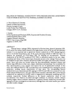
3. Results and Discussion 3.1. Climatic Condition during Different Growing Season Total annual precipitation during growing season was in the following order: 2015 (147.24 cm) > 2014 (111.07 cm) > 2013 (101.80 cm) > 2012 (68.55 cm). The 20-year average annual total precipitation was 113.49 cm (Figure 2). Year 2015 was the wettest as the total annual precipitation was higher than the 20-year average annual precipitation. In the Unites States, the year 2012 was considered as one of the worst drought years in the past 80 years or more, causing yields reductions of crops such as winter wheat, corn, and soybean [40,41]. The total monthly precipitation at the time of soybean planting during the June month in 2012 was 9.3 and 8.9 cm less compared to 2014 and 20-years average monthly precipitation. However, the monthly precipitation during the June month in 2014 was not significantly lower than 20-year average monthly precipitation. In 2014, the average monthly precipitation in month of April and May was 7.5 and 3.7 cm higher compared to 20-year average monthly precipitation. Total monthly precipitation in May at the time of corn planting in 2013 and 2015 was lower than the 20-year average monthly precipitation. However, the monthly precipitation in months after corn planting was higher in 2015 compared to 2013. In 2013, the monthly precipitation during the first three months after corn planting were similar providing more consistent soil moisture conditions for plant growth. In 2015, the precipitation in June was 11.13 and 10.18 cm higher compared to monthly precipitation in 2013 and 20-year average monthly precipitation. The higher soil moisture conditions in 2015 than 2013 after corn planting might have interfered with plant growth. The air temperatures during June in 2012 and 2014 at the time of soybean planting showed no big differences (Figure 2). In July, the air temperature was higher in 2012 than in 2014. The air temperatures in the month of May showed only small differences in 2013 and 2015. 3.2. Influence of Topographic Position on Corn and Soybean Yields There were no significant differences in soybean and corn yields among the three topographic positions in 2012 and 2013. The mean soybean and corn grain yields averaged over all topographic position in 2012 and 2013 were 3.32 and 11.21 Mg·ha−1 (Figure 4). In 2014, the soybean grain yield from depositional topographic position was significantly less than shoulder and backslope positions. Soybean yields from the depositional position was 38% lower from than yields from the shoulder position. The mean soybean yields averaged over all topographic positions was 2.59 Mg·ha−1 in 2014. Soybeans yields were lower in 2014 growing season than 2012 (Figure 4). In 2015, corn grain yields were significantly different at all three topographic positions. Corn grain yields at the deposition position were 62% and 52% lower than yields at shoulder and backslope positions, respectively. The backslope position resulted in 20% lower corn grain yields compared to the shoulder position in 2015. The annual variability in crop yields can be attributed to weather differences among years. Drier soil conditions resulting from lower precipitation during 2012 might have caused drought stress on soybeans causing lower yields overall, irrespective of topographic positions. The year 2015 was the wettest year compared to other years and may have resulted in different yields at all three topographic positions. Higher precipitation in April and May in 2014 (before soybean planting) as well as during May and June in 2015 resulted in excessive soil moisture conditions which may have caused waterlogging at the deposition position. The anaerobic soil conditions caused by the waterlogged soils resulted in poor plant stand establishment and growth and consequently, lowering grain yields in 2014 and 2015. Soybean is more sensitive to excessive soil moisture conditions compared to corn [42]. Crop yields were significantly different at topographic position in years with total annual precipitation equal or higher than 20-year average annual precipitation. Dry years showed no differences at various topographic positions. Many studies have shown yearly differences in crop yields due to topography [18,19,43–46]. In agreement with our results, Muñoz et al. [44] also reported that topography had major influence on corn yields during the year with higher precipitation. A study conducted by Halvorson and Doll [29] in eastern Oregon, Washington and
Agronomy 2016, 6, 57
8 of 22
North Dakota showed that landscape position and slope aspect significantly influences the grain yield of wheat. Jones et al. [47] reported that corn, sorghum and soybean yields were also affected by landscape positions and slope length. Thelemann et al. [48] observed that higher water retention for longer periods of time resulted in lower corn grain and stover yields at depositional and flat areas, whereas well drained summit positions had the highest yields as these slope positions drained earlier. Depression areas can accumulate water in turn they can impact corn and soybean yields and significant difference in yield can be observed during wet and dry years of precipitation in these areas [46]. Depth to B horizon can play an important role in regulating yields at different topographic positions. Khakural et al. [45] reported decreased yields of corn and soybean at backslope position compared to foot and upper toe slopes and concluded that it was due to eroded backslope positions. Based on the observed differences in rainfall patterns over 4 years, it is speculated that soil saturation in the early spring may be an important factor affecting differences in N availability to corn and soybean plants among the different landscape positions.
Figure 4. Corn and soybean grain yields at different topographic positions from 2012 to 2015. Same letter on bars indicate no significant differences at p < 0.05 according to Tukey-Kramer grouping test.
3.3. Influence of Topographic Position on ECa ECa-H-1, ECa-V-1 and ECa-V-0.5 were significantly lower at shoulder positions compared to backslope and deposition positions (Figure 5). ECa-H-0.5 showed significant differences at all three topographic positions, with the lowest value at shoulder position and highest values at deposition position. Topographic influence on ECa can be attributed to clay and soil moisture content at time of data collection. In a no-till corn/soybean fields low ECa values were observed at higher elevation compared to high ECa values at low elevation [49]. Brevik et al. [7] concluded that ECa may increase with an increase in volumetric water content due to strong relation (r2 = 0.70) between them. They also observed that higher elevation soil sampling locations had lower ECa values compared to lower elevations due to higher volumetric water content at lower elevation positions. Hanna et al. [50] observed soil moisture content during crop growth period using neutron probes and reported that within slope positions, soils on the foot slopes and backslopes contained on an average of 4 cm more
Agronomy 2016, 6, 57
9 of 22
available water than soils on the summits and shoulder slopes. Differences observed in soil moisture content may contribute towards variation in ECa values at different topographic position.
Figure 5. Influence of topographic positions on ECa sampled in October 2015 using EM38-MK2. Effective depth of electromagnetic field penetration for ECa-H-0.5, ECa-H-1, ECa-V-0.5 and ECa-V-1 were 0.45 m, 0.75 m, 0.75 m, and 1.5 m, respectively. Same letter on bars indicate no significant differences at p < 0.05 according to Tukey-Kramer grouping test.
3.4. Influence of Topographic Position on Soil Properties Sand content at depth 15–30 cm for shoulder position was significantly lower compared to deposition position (Table 1). Mean silt content at the deposition position was higher than shoulder and significantly higher than at the backslope position for both depths (Table 1). Mean clay content at depth 15–30 cm for the backslope position (31.874%) was greatest compared to other topographic positions. This could be due to higher percent slope change and more eroded top layer at the backslope position. The deposition position had significantly lower clay content at both depths compared to backslope and shoulder position (Table 1). At a depth of 15–30 cm, soil pH at the deposition position was significantly higher than the shoulder and backslope positions. However, no significant differences were obtained for soil pH for individual topographic positions between two depths. Total exchanges capacity was highest at the shoulder position at depth 15–30 cm compared to 0–15 cm depth at the shoulder and deposition positions as well as at 15–30 cm depth at the deposition position. At all topographic positions, OM, TN and TC were significantly lower at depth 15–30 cm compared to depth 0–15 cm. At 15–30 cm the deposition position had higher TN and TC than the shoulder and backslope position. Mehlich-3 P and Bray-1 P were significantly higher at 0–15 cm depth at the deposition position compared to other positions except at shoulder position from 0–15 cm depth. Significantly lower P concentrations were evident at the 15–30 cm depth at the backslope position. Physical removal of surface soil from steep slopes may decrease the concentration of N at shoulder position; however, it can rejuvenate the supply of rock derived nutrients such as P at shoulder positions [51]. At 15–30 cm depth, the shoulder and deposition position had similar Ca concentrations, which were significantly lower from Ca concentrations at
Agronomy 2016, 6, 57
10 of 22
backslope position from depth 0–15 cm. The Mg concentration at shoulder position from upper soil layer was significantly lower compared to backslope position Mg concentrations at both depths. Highest Mg concentration was obtained at backslope position from depth 15–30 cm, which was not significantly different to Mg concentration at 0–15 cm depth. The K concentrations were relatively higher at surface layers for all three topographic positions. Lowest K concentration was at 15–30 cm depth from deposition position, which was not significantly different from K concentrations from same depth at the shoulder position. The highest concentration of Na was obtained at the deposition position from depth 15–30 cm which was significantly higher than Na concentrations at 0–15 cm depth from all topographic positions and from 15–30 cm depth from the shoulder position. The S concentrations were significantly higher at the deposition position than both the shoulder and backslope positions for both depths. Concentration of Fe was significantly higher at the deposition position than the shoulder and backslope position for 15–30 cm depth. The highest Fe concentration was obtained within the surface layer of deposition position. The Al concentrations were significantly higher at the lower depth (15–30 cm) for all three topographic positions (Table 1). Backslope positions have significantly lower Mn concentrations at both depths compared to other two topographic positions. The B concentration showed no significant differences at all positions except at the backslope positon from depth 15–30 cm and at the deposition position at 0–15 cm depth. Surface layers have higher Cu concentrations compare to lower depth 15–30 cm. A study conducted by Wei et al. [52] found that deposition of eroded soil from upper positions into lower positions of landscape resulted in increase in TC, TN, silt and clay content from upper slope to foot slope along slope position gradients. An increase in soil organic carbon and total P from shoulder slope towards the toe slope in upper 25 cm depth of soil profile was observed by Heckrath et al. [53]. Yimer et al. [54] also reported significant differences in soil properties such as soil texture, soil pH, plant available phosphorus, CEC, exchangeable base cations, and percent base saturations. The differences were attributed to topographic aspect-induced microclimatic differences resulting in leaching and OM content differences within soil profile. Slope and aspect can determine the level and location of run-off and infiltration, which can influence the variation in water content and deposition of salts. Salts, pH, Na and CEC levels were observed to be greater in low elevation area when compared to high elevation areas [49]. Table 1. Changes in soil properties due to topographic positions at different depths. Shoulder Depth (cm) Sand, g·kg−1 Silt, g·kg−1 Clay, g·kg−1 pH TEC, meq/100 g OM, % TN, % TC, % P‡ mg·kg−1 Bray-1 P, mg·kg−1 Ca ‡ mg·kg−1 Mg ‡ mg·kg−1 K ‡ mg·kg−1 Na‡ mg·kg−1 S ‡ mg·kg−1 Fe ‡ mg·kg−1 Al ‡ mg·kg−1 Mn ‡ mg·kg−1 B ‡ mg·kg−1 Cu ‡ mg·kg−1
0–15 126.27 ab † 630.74 ab 242.99 cd 6.411 ab 12.969 c 1.988 a 0.106 a 1.064 a 41.444 ab 45.889 ab 1843.440 ab 135.670 c 157.780 a 25.833 c 9.111 c 149.720 cd 689.780 bc 159.670 a 0.591 ab 1.747 ab
15–30 95.81 b 618.38 abc 285.81 ab 5.928 b 15.637 abc 0.823 b 0.048 c 0.386 c 18.333 cd 15.500 c 1670.941 b 176.222 bc 89.778 cd 34.389 bc 14.278 c 125.834 d 894.781 a 70.611 bc 0.457a b 1.280 b
Topographic Position Backslope 0–15 15–30 124.12 ab 100.36 ab 593.89 bc 580.90 c 281.99 bc 318.74 a 6.144 ab 5.894 b 18.298 ab 20.845 a 2.073 a 0.809 b 0.107 a 0.044 c 1.084 a 0.381 c 28.167 bc 9.222 d 26.667 bc 4.944 c 2256.561 a 1962.728 ab 292.722 ab 419.56 a 152.610 a 103.280 bc 45.167 bc 92.722 ab 9.833 c 18.278 c 173.446 bc 130.561 d 751.564 b 941.835 a 89.944 b 36.000 c 0.569 ab 0.442 b 1.639 ab 1.184 b
Deposition 0–15 15–30 122.25 ab 132.25 a 652.10 a 640.02 a 225.65 d 227.73 d 6.433 ab 6.850 a 14.859 bc 13.183 bc 2.098 a 1.138 b 0.108 a 0.072 b 1.133 a 0.707 b 63.278 a 27.667 cbd 64.667 a 27.111 bc 1936.671 ab 1737.064 b 261.065 bc 286.111 abc 126.170 ab 66.056 d 92.000 b 134.390 a 28.222 a 36.278 a 278.561 a 196.941 b 599.285 c 626.332 c 139.786 a 159.226 a 0.669 a 0.649 ab 2.276 a 2.154 a
Means followed by the same letter within a row do not differ significantly at p < 0.05 according to Tukey-Kramer grouping test; ‡ Mehlich-3 extractable elements; Abbreviations: TEC, Total Exchange †
Agronomy 2016, 6, 57
11 of 22
Capacity; OM, Organic matter; TN, Total Nitrogen; TC, Total Carbon; P, Phosphorus; Mg, Magnesium; K, Potassium; Na, Sodium; S, Sulfur; Fe, Iron; Al, Aluminum; Mn, Manganese; Cu, Copper.
3.5. Correlation of ECa with Crop Grain Yields at Three Topographic Positions In 2013, corn grain yields were moderately correlated (r = ±0.50–±0.75) to ECa-H-0.5 at the shoulder position, and with ECa-H-1, ECa-V-0.5 and ECa-V-1 at the deposition (Table 2). Soybean grain yields showed no significant correlation with ECa at different topographic positions. However, soybean yields are weakly correlated (r < ±0.50) with ECa-H-0.5 and ECa-H-1 in 2012 and 2014 in all basins, when data are combined over all topographic positions. Soybean yields were also weakly correlated (r < ±0.50) with ECa-V-0.5 and ECa-V-1 in 2014. For the year 2015, both corn grain yields were weakly correlated (r < ±0.50) with ECa, when data was combined over all topographic positions. Kitchen et al. [4] concluded that ECa alone can explain corn and soybean yield variability (averaged over sites and years R2 = 0.21) better than topographic variables (averaged over sites and years R2 = 0.17). Two out of three research sites monitored for yield had weak correlations (r < ±0.50) with ECa averaged over three years [4]. Higher average annual precipitation during year 2015 (147.24 cm) and 2014 (111.07 cm) compared to 2013 (101.80 cm) and 2012 (68.55 cm) may have played an important role in contributing to soil moisture levels in 2015 and 2014, thus resulting in better correlations of ECa to yield. Kitchen et al. [5] concluded that precipitation received during the growing season for corn and soybeans may play an important role in governing ECa correlation to grain yields. Table 2. Correlation between ECa dipoles and soybean and corn grain yields.
Topographic Position
Crop Soybean
Shoulder Corn Soybean Backslope Corn Soybean Deposition Corn Soybean All Basins †† Corn
Year 2012 2014 2013 2015 2012 2014 2013 2015 2012 2014 2013 2015 2012 2014 2013 2015
Apparent Electrical Conductivity ECa-H-0.5 ECa-H-1 ECa-V-0.5 ECa-V-1 −0.208 0.060 0.397 0.230 0.278 −0.273 0.019 −0.372 0.606 * 0.066 0.072 0.168 0.105 0.138 0.001 0.122 −0.410 −0.378 −0.324 −0.250 −0.058 −0.286 −0.411 −0.331 −0.390 −0.331 −0.307 −0.251 0.121 −0.097 −0.136 −0.088 −0.284 −0.249 −0.106 −0.211 0.218 0.038 0.184 0.124 −0.374 −0.514 * −0.506 * −0.504 * −0.002 −0.263 −0.030 0.053 −0.276 * −0.265 * −0.141 −0.204 −0.381 * −0.489 * −0.449 * −0.494 * −0.118 −0.291 −0.252 −0.252 −0.464 * −0.522 * −0.479 * −0.475 *
* Significant at 0.05 probability level; †† All basins combined with no topographic separation.
3.6. Correlation of ECa with Soil Properties at Three Topographic Positions A moderate correlation (r = ±0.50–±0.75) was observed between ECa-H-0.5 and elevation with all basins without topographic separation (Table 3). However, no significant correlation was observed between ECa-H-0.5 and percent slope for all basins, and a weak correlation (r < ±0.50) was observed between ECa-H-0.5 and percent slope at the shoulder position. Correlation between ECa-H-0.5 and aspect at the shoulder position was moderate (r = ±0.50–±0.75) and for all basins with no topographic separation was weak (r < ±0.50). ECa-H-0.5 at 15–30 cm depth had a moderate (r = ±0.50–±0.75) correlation with sand at the shoulder position and weak correlation (r < ±0.50) with sand
Agronomy 2016, 6, 57
12 of 22
with all basins combined with no topographic separation. Weak and moderate correlation was observed between ECa-H-0.5 and silt at the backslope and deposition at 15–30 cm (Table 3). ECa-H-0.5 was weakly correlated (r < ±0.50) with soil pH from depth 0–15 cm and TEC from depth 15–30 cm, respectively at the deposition position. Combining the data for all topographic positions resulted in weak correlation (r < ±0.50) of ECa-H-0.5 with soil pH at 15–30 cm depth as well as with TEC at depth 0–15 cm. ECa-H-0.5 was moderately correlated (r = ±0.50–±0.75) with OM, Ca and S at the depositional position for depth 0–15 cm. ECa-H-0.5 showed weak negative correlation with Al at the deposition position at a depth of 15–30 cm. The negative correlation of Al increased, whereas the positive correlation of Ca and S decreased with ECa-H-0.5 when data were combined over all topographic positions. At the backslope position, TN, TC and Mg showed moderate correlation (r = ±0.50–±0.75) with ECa-H-0.5 for depth 15–30 cm. Total N and TC was negatively correlated with ECa-H-0.5 at this depth. Mg showed positive and weak correlation for depth 0–15 cm, which improved to moderate correlation (r = ±0.50–±0.75) if analyzed in absence of any topographic positions. When data were analyzed by removing the topographic positions, the correlations of Na was improved and resulted in moderate correlation (r = ±0.50–±0.75) with ECa-H-0.5. Mehlich-3 P and Bray-1 P showed a moderate (r = ±0.50–±0.75) and a moderate to strong correlation (r > ±0.75) with ECa-H-0.5 for 0–15 cm and 15–30 cm soil depth at the shoulder position, respectively. However, the correlations decreased to weak (r < ±0.50) when Mehlich-3 P and Bray-1 P were analyzed by combining data over topographic positions. At the shoulder position only, Fe, Ca and Cu showed a significant positive correlation with ECa-H-0.5. The correlation of ECa-H-0.5 with Fe and Cu decreases when data were combined for all topographic positions. The correlation of S at shoulder position with ECa-H-0.5 reversed when data were combined over all topographic positions. The significant positive correlations of ECa-H-1 was obtained for elevation at the deposition position and the following soil properties: soil pH at deposition positions; clay at the shoulder position for depth 0–15 cm; TEC at the shoulder positions for both depths; Mehlich-3 P, Bray-1 P, and Cu at the shoulder position for both depths; Mg at all three topographic positions for both depths; Na at the backslope position for both depths; S at the deposition position for both depths; K and Fe at depth 15–30 cm and Ca at depth 0–15 cm for the shoulder position; Ca and Na at depth 15– 30 cm and K at depth 0–15 cm for deposition positions (Table 4). The correlation of ECa-H-1 decreased for all ions except Mg and Na. No significant correlation was obtained for Mehlich-3 P and Bray-1 P when data were combined over all topographic positions. Al at 0–15 cm and Fe and Mn at depth 15–30 only showed weak correlations (r < ±0.50) with ECa-H-1 when data were combined over topographic positions. The significant and positive correlations of ECa-V-0.5 was obtained for following soil properties: soil pH at all three topographic positions; Mehlich-3 P, Bray-1 P, Ca, Fe and Cu at the shoulder position for both depths; B at the shoulder position at depth 0–15 cm (r > ±75); Mg at backslope and deposition positions for both depths; Al, Mn and soil pH at depth 15–30 cm for backslope positions; Na at the backslope position; Ca, Na and Fe at the deposition positions at 15–30 cm (Table 5). Correlations with ECa-V-0.5 decreased for Cu, Mn, Fe, Na and Ca, when data were combined over topographic positions. Correlation improved for Mg at depth 0.15 cm. Correlation of ECa-V-0.5 with TEC and S were only obtained when data was combined over topographic positions. The soil properties that showed significant correlations with ECa-V-1 were sand at the deposition position at 0–15 cm deep (r = ±0.50–±0.75); silt at backslope and deposition for 0–15 cm depth (r < ±0.50); clay at the shoulder position at 0–015 cm (r = ±0.50–±0.75); TEC, Mehlich-3 P, Bray-1 P, and Cu at shoulder positions for both depths; Mg at all three topographic positions; Fe and K from depth 15–30 cm and Ca at depth 0–15 cm at the shoulder position; Soil pH at depth 15–30 cm for backslope and deposition positions; Al and Mn at the backslope position from depth 15–30 cm; Na at the backslope position; Ca and Fe at the deposition position from depth 15–30 cm (Table 6). The correlations with ECa-V-1 improved only for Al, Fe at the deposition position and Mg at the shoulder and deposition position when data was combined over topographic positions. Table 3. Correlation coefficient between soil properties and ECa-H-0.5.
Agronomy 2016, 6, 57
Properties Elevation, m Slope, % Aspect, degree Sand, g·kg−1 Silt, g·kg−1 Clay, g·kg−1 pH (1:1 H2O) TEC, meq/100 g OM, % TN, % TC, % P ‡, mg·kg−1 Bray-1 P, mg·kg−1 Ca ‡, mg·kg−1 Mg ‡, mg·kg−1 K ‡, mg·kg−1 Na ‡, mg·kg−1 S ‡, mg·kg−1 Fe ‡, mg·kg−1 Al ‡, mg·kg−1 Mn ‡, mg·kg−1 B ‡, mg·kg−1 Cu ‡, mg·kg−1
13 of 22
Depth (cm)
0–15 15–30 0–15 15–30 0–15 15–30 0–15 15–30 0–15 15–30 0–15 15–30 0–15 15–30 0–15 15–30 0–15 15–30 0–15 15–30 0–15 15–30 0–15 15–30 0–15 15–30 0–15 15–30 0–15 15–30 0–15 15–30 0–15 15–30 0–15 15–30 0–15 15–30 0–15 15–30
Shoulder n = 18 −0.376 0.447 0.578 −0.409 0.654 * 0.063 −0.159 0.266 −0.336 0.140 0.374 0.396 0.179 0.029 0.120 −0.153 0.069 −0.238 0.082 0.670 * 0.806 * 0.580 * 0.763 * 0.274 0.736 * 0.456 * 0.446 * −0.354 0.205 0.253 0.206 0.006 −0.590 * 0.794 * 0.600 * −0.121 −0.331 0.231 0.366 0.337 0.397 0.482 * 0.528 *
Apparent ECa-H-0.5 Backslope n = 18 Deposition n = 18 0.137 0.143 0.075 −0.098 −0.409 −0.295 0.242 0.256 0.298 −0.271 −0.353 −0.285 −0.507 * 0.492 * 0.123 0.071 0.358 −0.216 −0.096 0.482 * 0.015 0.419 0.359 0.190 0.349 −0.463 * −0.198 0.533 * −0.448 0.227 −0.277 0.180 −0.564 * 0.143 −0.287 0.255 −0.558 * 0.171 -0.360 0.355 0.214 0.234 −0.383 0.328 0.122 0.244 0.095 0.500 * 0.246 −0.287 0.477 * 0.338 0.690 * 0.066 0.128 0.351 0.408 0.039 0.393 0.131 0.473 * −0.088 0.000 0.500 * 0.255 0.442 −0.158 0.013 0.294 −0.064 0.399 −0.269 −0.019 −0.470 * −0.046 0.114 0.066 0.103 −0.059 0.180 0.065 0.211 −0.119 0.348 0.091 0.277
All Basins †† n = 54 −0.647 * 0.093 −0.362 * −0.017 0.333 * −0.066 −0.015 0.079 −0.208 0.060 0.396 * 0.448 * 0.092 0.121 0.215 −0.045 0.199 0.022 0.262 * 0.296 * 0.273 * 0.228 0.285 * 0.292 * 0.292 * 0.616 * 0.519 * −0.245 −0.020 0.532* 0.536 * 0.459 * 0.360 * 0.511 * 0.509 * −0.121 −0.423 * −0.143 0.358 * 0.194 0.350 * 0.371 * 0.490 *
All basins combined with no topographic separation; Abbreviations: TEC, Total Exchange Capacity; OM, Organic matter; TN, Total Nitrogen; TC, Total Carbon; P, Phosphorus; Mg, Magnesium; K, Potassium; Na, Sodium; S, Sulfur; Fe, Iron; Al, Aluminum; Mn, Manganese; Cu, Copper; ‡ Mehlich-3 extractable elements; * Significant at 0.05 probability level.
††
Agronomy 2016, 6, 57
14 of 22
Table 4. Correlation coefficient between soil properties and ECa-H-1. Properties Elevation, m Slope, % Aspect, degree Sand, g·kg−1 Silt, g·kg−1 Clay, g·kg−1 pH (1:1 H2O) TEC, meq/100 g OM, % TN, % TC, % P ‡, mg·kg−1 Bray-1 P, mg·kg−1 Ca ‡, mg·kg−1 Mg ‡, mg·kg−1 K ‡, mg·kg−1 Na ‡, mg kg−1 S ‡, mg·kg−1 Fe ‡, mg·kg−1 Al ‡, mg·kg−1 Mn ‡, mg·kg−1 B ‡, mg·kg−1 Cu‡, mg·kg−1
Depth (cm)
0–15 15–30 0–15 15-30 0–15 15–30 0–15 15–30 0-15 15–30 0–15 15–30 0–15 15–30 0–15 15–30 0–15 15–30 0–15 15–30 0–15 15-30 0-15 15–30 0–15 15–30 0–15 15–30 0–15 15–30 0–15 15–30 0–15 15–30 0–15 15–30 0–15 15–30 0–15 15–30
Shoulder n = 18 0.038 0.394 0.075 −0.405 0.142 −0.284 −0.433 0.575 * 0.377 0.429 0.043 0.544 * 0.470 * 0.307 −0.105 −0.271 −0.264 −0.295 −0.267 0.570 * 0.484 * 0.573 * 0.458 * 0.614 * 0.386 0.592 * 0.588 * 0.077 0.580 * 0.052 0.347 0.031 0.230 0.440 0.523 * −0.127 0.148 −0.121 0.000 0.323 −0.105 0.500 * 0.537 *
Apparent ECa-H-1 Backslope n = 18 Deposition n = 18 0.122 0.368 * 0.034 −0.234 −0.100 0.036 0.189 0.210 0.257 −0.376 −0.538 * −0.260 −0.012 0.142 0.334 0.089 −0.111 0.296 0.053 0.347 0.411 0.474 * 0.209 0.224 −0.113 −0.235 0.053 0.021 −0.434 −0.165 −0.135 0.029 −0.305 −0.127 −0.097 0.011 −0.286 −0.100 0.040 0.024 −0.166 −0.155 0.086 −0.034 −0.155 −0.182 0.024 0.060 0.031 −0.494 * 0.536 * 0.610 * 0.595 * 0.471 * 0.065 0.510 * −0.112 −0.113 0.568 * 0.549 0.665 * 0.488 * 0.296 0.501 * 0.268 0.492 * −0.042 −0.043 −0.004 −0.262 0.084 0.046 −0.383 −0.218 −0.302 −0.094 0.352 −0.261 0.076 0.121 0.201 0.074 0.232 −0.060 −0.068 0.113
All Basins †† n = 54 −0.568 * 0.086 −0.327 * 0.016 0.144 −0.215 −0.020 0.206 −0.078 0.107 0.403 * 0.475 * 0.060 0.168 0.088 −0.042 0.114 0.025 0.189 0.177 0.029 0.122 0.044 0.304 * 0.144 0.708 * 0.595* −0.101 −0.056 0.640 * 0.707 * 0.463 * 0.460 * 0.436 * 0.331 * −0.095 −0.348 * −0.344 * 0.195 0.176 0.221 0.278 * 0.373 *
All basins combined with no topographic separation; Abbreviations: TEC, Total Exchange Capacity; OM, Organic matter; TN, Total Nitrogen; TC, Total Carbon; P, Phosphorus; Mg, Magnesium; K, Potassium; Na, Sodium; S, Sulfur; Fe, Iron; Al, Aluminum; Mn, Manganese; Cu, Copper; ‡ Mehlich-3 extractable elements; * Significant at 0.05 probability level.
††
Table 5. Correlation coefficient between soil properties and ECa-V-0.5. Properties Elevation, m Slope, % Aspect, degree Sand, g·kg−1 Silt, g·kg−1 Clay, g·kg−1
Depth (cm)
0–15 15–30 0–15 15–30 0–15
Shoulder n = 18 −0.028 0.319 0.267 −0.119 0.289 −0.129 −0.362 0.210
Apparent ECa-V-0.5 Backslope n = 18 Deposition n = 18 0.158 0.551 * −0.009 0.013 −0.148 −0.060 0.073 0.539 * 0.225 −0.365 −0.483 * −0.419 0.099 0.047 0.378 −0.055
All Basins †† n = 54 −0.506 * 0.074 −0.291 * 0.103 0.195 −0.186 0.005 0.113
Agronomy 2016, 6, 57
pH (1:1 H2O) TEC, meq/100 g OM, % TN, % TC, % P ‡, mg·kg−1 Bray-1 P, mg·kg−1 Ca ‡, mg·kg−1 Mg ‡, mg·kg−1 K ‡, mg·kg−1 Na ‡, mg·kg−1 S ‡, mg·kg−1 Fe ‡, mg kg−1 Al ‡, mg kg−1 Mn ‡, mg·kg−1 B ‡, mg·kg−1 Cu ‡, mg·kg−1
15 of 22 15–30 0–15 15–30 0–15 15–30 0–15 15–30 0–15 15–30 0–15 15–30 0–15 15–30 0–15 15–30 0–15 15–30 0–15 15–30 0–15 15–30 0–15 15–30 0–15 15–30 0–15 15–30 0–15 15–30 0–15 15–30 0–15 15–30 0–15 15–30
0.181 0.601 * 0.338 0.422 0.240 0.266 −0.141 −0.188 −0.177 −0.243 −0.189 0.724 * 0.573 * 0.782 * 0.580 * 0.655 * 0.469 * 0.376 0.329 0.049 0.327 0.357 0.062 0.239 −0.053 0.491 * 0.461 −0.299 −0.145 0.346 0.146 0.770 * 0.212 0.821 * 0.580 *
−0.206 −0.001 0.488 * 0.250 −0.157 0.007 −0.423 −0.094 −0.307 −0.078 −0.287 0.060 −0.125 0.093 −0.100 0.041 0.082 0.532 * 0.582 * 0.056 −0.141 0.660 * 0.747 * 0.247 0.300 −0.048 −0.010 0.093 −0.506 * −0.215 0.532 * −0.035 0.230 0.283 0.004
0.388 0.450 * 0.504 * −0.096 −0.060 −0.062 −0.324 −0.077 −0.068 −0.121 −0.042 −0.018 −0.183 −0.061 −0.208 −0.090 −0.497 * 0.459 * 0.568 * 0.440 0.010 0.372 0.573 * 0.287 0.414 −0.268 −0.541 * 0.141 0.130 −0.103 −0.159 0.030 0.166 −0.100 −0.104
−0.134 0.196 0.501 * 0.399 * 0.000 0.136 0.042 −0.061 0.124 −0.015 0.188 0.241 0.081 0.214 0.106 0.302 * 0.167 0.624 * 0.542 * −0.116 −0.097 0.605 * 0.723 * 0.384 * 0.399 * 0.398 * 0.304 * −0.139 −0.409 * −0.164 0.285 * 0.264 * 0.316 * 0.425 * 0.391 *
All basins combined with no topographic separation; Abbreviations: TEC, Total Exchange Capacity; OM, Organic matter; TN, Total Nitrogen; TC, Total Carbon; P, Phosphorus; Mg, Magnesium; K, Potassium; Na, Sodium; S, Sulfur; Fe, Iron; Al, Aluminum; Mn, Manganese; Cu, Copper; ‡ Mehlich-3 extractable elements; * Significant at 0.05 probability level.
††
Table 6. Correlation coefficient between soil properties and ECa-V-1. Properties Elevation, m Slope, % Aspect, degree Sand, g·kg−1 Silt, g·kg−1 Clay, g·kg−1 pH (1:1 H2O) TEC, meq/100 g OM, % TN, % TC, % P ‡, mg·kg−1
Depth (cm)
0–15 15–30 0–15 15–30 0–15 15–30 0–15 15–30 0–15 15–30 0–15 15–30 0–15 15–30 0–15 15–30 0–15
Shoulder n = 18 −0.089 0.392 −0.020 −0.228 0.074 −0.423 −0.337 0.561 * 0.322 0.446 0.010 0.550 * 0.460 * 0.407 0.063 −0.229 −0.143 −0.241 −0.158 0.60 *
Apparent ECa-V-1 Backslope n = 18 Deposition n = 18 0.191 0.562 * −0.075 −0.075 −0.150 −0.058 0.099 0.539 * 0.197 −0.319 −0.491 * −0.490 * 0.100 0.116 0.364 0.025 −0.194 0.256 0.021 0.371 0.493 * 0.507 * 0.182 −0.143 −0.165 −0.207 0.014 0.064 −0.436 −0.257 −0.074 0.030 −0.272 −0.125 −0.047 −0.014 −0.260 −0.083 0.041 0.030
All Basins †† n = 54 −0.540 * 0.028 −0.368 * 0.132 0.147 −0.244 0.058 0.151 −0.150 0.112 0.455 * 0.373 * −0.006 0.163 0.099 −0.014 0.151 0.048 0.223 0.192
Agronomy 2016, 6, 57
Bray-1 P, mg·kg−1 Ca ‡, mg·kg−1 Mg ‡, mg·kg−1 K ‡, mg·kg−1 Na ‡, mg·kg−1 S‡, mg·kg−1 Fe‡, mg·kg−1 Al‡, mg·kg−1 Mn‡, mg·kg−1 B‡, mg·kg−1 Cu‡, mg·kg−1
16 of 22 15–30 0–15 15–30 0–15 15–30 0–15 15–30 0–15 15–30 0–15 15–30 0–15 15–30 0–15 15–30 0–15 15–30 0–15 15–30 0–15 15–30 0–15 15–30
0.440 * 0.611 * 0.492 * 0.682 * 0.287 0.550 * 0.494 * 0.126 0.454 * 0.009 0.274 0.001 0.315 0.415 0.493 * 0.000 0.105 −0.059 0.121 0.310 −0.047 0.556 * 0.645 *
−0.149 0.076 −0.127 0.026 0.102 0.468 * 0.559 * 0.043 −0.129 0.610 * 0.723 * 0.228 0.260 −0.082 −0.022 0.091 −0.470 * −0.185 0.533 * −0.010 0.258 0.262 0.001
−0.071 0.006 −0.091 −0.062 −0.475 * 0.316 * 0.456 * 0.403 0.057 0.209 0.440 0.167 0.305 −0.329 −0.570 * 0.133 0.077 −0.121 −0.097 −0.085 0.074 −0.071 −0.133
0.064 0.145 0.089 0.246 0.131 0.608 * 0.538 * −0.123 −0.116 0.582 * 0.732 * 0.379 * 0.420 * 0.377 * 0.263 * −0.086 −0.380 * −0.281 * 0.287 * 0.105 0.265 * 0.286 * 0.356 *
All basins combined with no topographic separation; Abbreviations: TEC, Total Exchange Capacity; OM, Organic matter; TN, Total Nitrogen; TC, Total Carbon; P, Phosphorus; Mg, Magnesium; K, Potassium; Na, Sodium; S, Sulfur; Fe, Iron; Al, Aluminum; Mn, Manganese; Cu, Copper; ‡ Mehlich-3 extractable elements; * Significant at 0.05 probability level.
††
Topographic and landscape properties including elevation, slope, curvature and aspect were weakly correlated (r < ±0.50) to ECa (shallow and deep) for three different soil textures [4]. Elevation was negatively correlated to ECa when all basins were combine together and our results were in agreement with results observed by Peralta and Costa [49]. Results from a multi-state dataset collected by Sudduth et al. [6] on ECa and soil properties showed weak to moderate correlations of ECa with clay content and CEC across most fields. Correlations of ECa with other soil properties including soil moisture, silt, sand, organic C and paste EC were lower and more variable for the fields across North-central USA [6]. A positive correlation between ECa and clay content was observed at four of six sites in southern high plains of Texas [16]. Clay content was not significantly correlated to ECa except for ECa-H-1 and ECa-V-1 at 0–15 cm depth on shoulder position at our research site. In another study, conducted by Carroll and Oliver [13] moderate and moderate to strong correlation were observed between ECa and soil textural fractions (sand, silt and clay) at two separate research sites. The relations between ECa and the topsoil properties were stronger than those for the subsoil. A negative correlation was observed for sand and bulk density with ECa as large bulk densities were associated with sandy soil [13]. Heil and Schmidhalter [55] investigated spatial distribution of clay, silt, and sand/gravel on highly variable landscape in Germany and concluded that clay and sand/gravel were most closely related to the ECa, and observed R2 values ranging between 0.67 and 0.76. Jung et al. [3] observed a significant positive correlation of ECa with clay content at 15–30 cm depth and a negative correlation with silt and a weak correlation of ECa with sand. Many studies reported a correlation between cation exchange capacity and ECa, which can be attributed to clay content in a soil profile [3,6,16]. No significant results were observed in our research study when OM was correlated to ECa in all basins with no topographic separation (Table 3). In contrast, OM distribution showed highly variable and weak correlation with ECa in study conducted by Sudduth et al. [6] and by Omonode and Vyn [56]. A significant Pearson correlation coefficient of r > 0.70 indicated that ECa could be used to estimate P and K levels [57] and can be used to map the levels of these nutrients with minimum error [58]. However, weak (r < ±50) correlations were observed for ECa with all basins with no topographic separations for Mehlich-3 P
Agronomy 2016, 6, 57
17 of 22
and Bray-1 P. Similar results of weak correlation of ECa with P were observed by [3,56,57] for surface soil horizons. When data were separated on topographic positions, a moderate to strong correlation was observed between ECa and Mehlich-3 P, and Bray-1 P for 15–30 cm depth and could be explained by an increased P adsorption to clay content with increasing depth [3]. No significant correlations were found between ECa and TN, and TC in claypan soils of Missouri [3]. However, Peralta and Costa [49] and Neely et al. [59] observed strong negative correlation of ECa with soil organic matter and inorganic carbon in coarse-loamy Mollisols and clayey Vertisols, respectively. Calcium, Mg and Na were often positively and moderately to strongly correlated to ECa [16,58]. Soils at our southern Illinois study sites are in the Hosmer series and are characterized by an Ochric epipedon followed by an argillic horizon, occasional occurrence of fragipans and a fairly well distribution of Ca on all topographic positions (Table 1). Stronger correlation of ECa with Ca may be explained by its significant distribution over the study site. Electromagnetic techniques have been well noted for mapping of salt-affected soils [60]. Salts of Na can be an important contributor to salinity in southern and central Illinois and electromagnetic induction techniques have been widely used in mapping these salt affected soils [61–64] and a moderate to strong correlation was observed at our research site. 3.7. Spatial Interpolation of Selected Soil Properties and ECa A close relation between ECa and soil properties can be obtained to develop spatially interpolated maps. Significant influence of topographic positions on some soil properties could make it difficult to make accurate soil maps from ECa. To meet our second objective, we have presented two different case scenarios for modeling Mehlich-3 P and Mehlich-3 Na with ECa-H-0.5 at 0–15 cm depth and ECa-V-1 at 15–30 cm, respectively. All modeling parameters and cross validation RMSE are presented in Table 7. Spatial interpolation between Mehlich-3 P and ECa-H-0.5 with all topographic positions combined together in all basins resulted in larger cross validation RMSE compared to shoulder and backslope positions. Cross validation RMSE between Mehlich-3 Na and ECa-V-1 for all basins, backslope and deposition positions were zero. Correlation was moderate (r = ±0.50–±0.75) for Mehlich-3 P and ECa-H-0.5 at the shoulder position and for Mehlich-3 Na and ECa-V-1 in all basins with no topographic separation and backslope position (Table 7). Weak correlation (r < ±0.50) was observed between Mehlich-3 P and ECa-H-0.5 at all basins, backslope and deposition and between Mehlich-3 Na and ECa-V-1 at shoulder and deposition. Splitting data on soil topographic position results in changing correlation among datasets. This can be explained by the change in spatial resolution of the data set where modifiable areal unit problem (MUAP) can occur [63,65,66]. Modeling Mehlich-3 P data splitting on basis of topographic positions can improve correlation and spatial interpolation while reducing cross validation RMSE. Splitting of Mehlich-3 Na dataset results in lower correlation among data sets which may increase cross validation RMSE. It depends on study objectives as well as on the level of details at which prediction maps are needed. Methods of delineation topography presented in this paper and developing separate soil maps on basis of topographic positions can certainly improve level of details for site-specific management and results presented in this paper can be easily replicated. The ECa measurement as carried out by the combination of a GPS system and an EM38-MK2 device is a simple, fast, and low-cost method to obtain spatial soil information with high resolution. In areas where significant landscape (elevation/topographic) induced variation occur in soil properties, splitting ECa survey data can certainly improve our understanding of spatial distribution of available nutrients.
Agronomy 2016, 6, 57
18 of 22
Table 7. Spatial interpolation of Mehlich-3 phosphorus with ECa-H-0.5 at 0–15 cm depth and Mehlich-3 sodium with ECa-V-1 at 15–30 cm depth. Data Type
Interpolation Method Simple Cokring
n 54
Shoulder
Simple Cokring
18
Backslope
Simple Cokring
18
Deposition
Simple Cokring
18
Simple Cokring
54
Shoulder
Simple Cokring
18
Backslope
Simple Cokring
18
Deposition
Simple Cokring
18
All Basins ‡
All Basins
‡
Datasets Used Mehlich-3 P ECa-H-0.5 Mehlich-3 P ECa-H-0.5 Mehlich-3 P ECa-H-0.5 Mehlich-3 P ECa-H-0.5 Mehlich-3 Na ECa-V-1 Mehlich-3 Na ECa-V-1 Mehlich-3 Na ECa-V-1 Mehlich-3 Na ECa-V-1
Correlation among Datasets 0.296 * 0.670 * −0.360 ** 0.375 ** 0.732 * 0.274 0.723 * 0.440 **
Nugget 0.232 0.380 0.644 0.523 0.026 0.396 0.685 0.723 0.000 0.000 0.467 0.400 0.000 0.000 0.000 0.523
Model Pentaspherical
Lag Size 27.104
No. of Lags 12
RMSE 26.962
Cross-Validation RMSE 11.428
Exponential
30.399
12
14.458
11.369
Exponential
79.321
12
11.591
0.432
Exponential
100.654
12
33.866
32.689
Exponential
30.734
12
42.972
0.000
Exponential
32.894
12
10.813
5.321
K-Bessell
47.540
12
56.951
0.000
Exponential
99.831
12
47.286
0.000
All basins combined with no topographic separation; * Significant at 0.05 probability level; ** Significant at 0.10 probability level.
Agronomy 2016, 6, 57
19 of 22
4. Conclusions Crop grain yields and soil properties were affected by the topography at a watershed scale. Corn and soybean yields were significantly lower at deposition positions in wet years compared to years with average rainfall. The influence of topography on crop yields varies annually due to yearly variation in weather conditions. Available elements in soil were highly variable with topographic position. Topographic differences resulted in soil water movement and sediments deposition from upper to lower slope position that contribute to variation in available elements in soil at different depths and topographic positions. Slope variation from 1%–20% at the research site had a strong influence on soil properties at watershed scale. ECa was also influenced by topographic positions where higher ECa was observed at deposition positions in both vertical and horizontal mode of operations. Correlation of ECa can provide important information of spatial distribution of soil properties and help in site-specific management. Significant correlations were found between ECa and some soil properties (sand, silt, TEC, OM, P, Ca, Mg, Na). It is important to consider topography in any spatial modeling and mapping where large slope change can interact and govern spatial distribution of soil properties and crop yields. Correlation of ECa with soil properties can be positive and negative when data is divided on basis of topographic positions. In spatial mapping of Mehlich-3 P, correlation with ECa decreased when there was no topographic separation, whereas for Mehlich-3 Na correlation with ECa was generally improved. Correlation between ECa and available elements can be influenced by topographic position. If the user is interested in details of managing elements, separate interpolation models should be developed for elements like P. However, if high correlations exist between soil properties and ECa on a whole field scale without any topographic influence, single interpolation model can be developed (e.g., Na in the current study). Advantage of the ECa based soil survey is the high number of ECa measurements per unit area. It is possible to create maps with a very high spatial resolution, as needed for precision farming or generally for a site specific soil use and management. Methods of delineating topography positions presented in this paper can easily be replicated on other fields with similar landscape characteristics. High resolution topographic position and site specific management or productivity maps can be produced using ECa survey data. Furthermore, with availability of variable rate planters, sprayers and fertilizer applicators these high resolution maps can be integrated for effective and cost efficient management plans for crop production. Acknowledgments: We thank the reviewers for their valuable comments and suggestions to improve the quality of this manuscript. We are grateful to our funding sources, McIntire-Stennis Cooperative Forest Research Program and Illinois Nutrient Research & Education Council. Author Contributions: Gurbir Singh was responsible for management of the project, data collection, statistical analysis, interpretation of results and manuscript preparation. Karl W. J. Williard and Jon E. Schoonover were involved in manuscript editing. Conflicts of Interest: The authors declare no conflict of interest.
References 1. 2.
3. 4. 5.
Doolittle, J.A.; Brevik, E.C. The use of electromagnetic induction techniques in soils studies. Geoderma 2014, 223, 33–45. Jiang, P.; Anderson, S.H.; Kitchen, N.R.; Sudduth, K.A.; Sadler, E.J. Estimating plant-available water capacity for claypan landscapes using apparent electrical conductivity. Soil Sci. Soc. Am. J. 2007, 71, 1902– 1908. Jung, W.; Kitchen, N.; Sudduth, K.; Kremer, R.; Motavalli, P. Relationship of apparent soil electrical conductivity to claypan soil properties. Soil Sci. Soc. Am. J. 2005, 69, 883–892. Kitchen, N.; Drummond, S.; Lund, E.; Sudduth, K.; Buchleiter, G. Soil electrical conductivity and topography related to yield for three contrasting soil-crop systems. Agron. J. 2003, 95, 483–495. Kitchen, N.; Sudduth, K.; Myers, D.; Drummond, S.; Hong, S. Delineating productivity zones on claypan soil fields using apparent soil electrical conductivity. Comput. Electron. Agric. 2005, 46, 285–308.
Agronomy 2016, 6, x FOR PEER REVIEW
6.
7. 8. 9. 10. 11. 12. 13. 14. 15. 16.
17. 18. 19. 20.
21. 22. 23. 24. 25. 26. 27. 28. 29. 30.
20 of 22
Sudduth, K.; Kitchen, N.; Wiebold, W.; Batchelor, W.; Bollero, G.; Bullock, D.; Clay, D.; Palm, H.; Pierce, F.; Schuler, R. Relating apparent electrical conductivity to soil properties across the north-central USA. Comput. Electron. Agric. 2005, 46, 263–283. Brevik, E.C.; Fenton, T.E.; Lazari, A. Soil electrical conductivity as a function of soil water content and implications for soil mapping. Precis. Agric. 2006, 7, 393–404. Kitchen, N.; Sudduth, K.; Drummond, S. Soil electrical conductivity as a crop productivity measure for claypan soils. J. Prod. Agric. 1999, 12, 607–617. Kravchenko, A.N.; Thelen, K.; Bullock, D.; Miller, N. Relationship among crop grain yield, topography, and soil electrical conductivity studied with cross-correlograms. Agron. J. 2003, 95, 1132–1139. Sudduth, K.; Drummond, S.; Kitchen, N. Accuracy issues in electromagnetic induction sensing of soil electrical conductivity for precision agriculture. Comput. Electron. Agric. 2001, 31, 239–264. Doolittle, J.; Sudduth, K.; Kitchen, N.; Indorante, S. Estimating depths to claypans using electromagnetic induction methods. J. Soil Water Conserv. 1994, 49, 572–575. Corwin, D.; Lesch, S. Apparent soil electrical conductivity measurements in agriculture. Comput. Electron. Agric. 2005, 46, 11–43. Carroll, Z.; Oliver, M. Exploring the spatial relations between soil physical properties and apparent electrical conductivity. Geoderma 2005, 128, 354–374. Sudduth, K.A.; Kitchen, N.; Bollero, G.; Bullock, D.; Wiebold, W. Comparison of electromagnetic induction and direct sensing of soil electrical conductivity. Agron. J. 2003, 95, 472–482. Inman, D.J.; Freeland, R.S.; Ammons, J.T.; Yoder, R.E. Soil investigations using electromagnetic induction and ground-penetrating radar in southwest tennessee. Soil Sci. Soc. Am. J. 2002, 66, 206–211. Bronson, K.; Booker, J.; Officer, S.; Lascano, R.; Maas, S.; Searcy, S.; Booker, J. Apparent electrical conductivity, soil properties and spatial covariance in the U.S. Southern high plains. Precis. Agric. 2005, 6, 297–311. Brevik, E.C.; Fenton, T.E. The effect of changes in bulk density on soil electrical conductivity as measured with the geonics em-38. Soil Horiz. 2004, 45, 96–102. Jiang, P.; Thelen, K. Effect of soil and topographic properties on crop yield in a north-central corn– soybean cropping system. Agron. J. 2004, 96, 252–258. Kravchenko, A.N.; Bullock, D.G. Correlation of corn and soybean grain yield with topography and soil properties. Agron. J. 2000, 92, 75–83. McVay, K.; Budde, J.; Fabrizzi, K.; Mikha, M.; Rice, C.; Schlegel, A.; Peterson, D.; Sweeney, D.; Thompson, C. Management effects on soil physical properties in long-term tillage studies in kansas. Soil Sci. Soc. Am. J. 2006, 70, 434–438. Sariyildiz, T.; Anderson, J.; Kucuk, M. Effects of tree species and topography on soil chemistry, litter quality, and decomposition in northeast turkey. Soil Biol. Biochem. 2005, 37, 1695–1706. Gregorich, E.; Greer, K.; Anderson, D.; Liang, B. Carbon distribution and losses: Erosion and deposition effects. Soil Tillage Res. 1998, 47, 291–302. Kang, S.; Doh, S.; Lee, D.; Lee, D.; Jin, V.L.; Kimball, J.S. Topographic and climatic controls on soil respiration in six temperate mixed-hardwood forest slopes, korea. Glob. Chang. Biol. 2003, 9, 1427–1437. Moore, I.D.; Gessler, P.; Nielsen, G.; Peterson, G. Soil attribute prediction using terrain analysis. Soil Sci. Soc. Am. J. 1993, 57, 443–452. Ritchie, J.C.; McCarty, G.W.; Venteris, E.R.; Kaspar, T. Soil and soil organic carbon redistribution on the landscape. Geomo 2007, 89, 163–171. Zhu, Q.; Lin, H. Influences of soil, terrain, and crop growth on soil moisture variation from transect to farm scales. Geoderma 2011, 163, 45–54. Zhu, Q.; Schmidt, J.P.; Bryant, R.B. Maize (Zeamays l) yield response to nitrogen as influenced by spatio-temporal variations of soil-water-topography dynamics. Soil Tillage Res. 2015, 146, 174–183. Florinsky, I.V.; Eilers, R.G.; Manning, G.; Fuller, L. Prediction of soil properties by digital terrain modelling. Environ. Model. Softw. 2002, 17, 295–311. Halvorson, G.A.; Doll, E. Topographic effects on spring wheat yields and water use. Soil Sci. Soc. Am. J. 1991, 55, 1680–1685. Huang, X.; Wang, L.; Yang, L.; Kravchenko, A.N. Management effects on relationships of crop yields with topography represented by wetness index and precipitation. Agron. J. 2008, 100, 1463–1471.
Agronomy 2016, 6, x FOR PEER REVIEW
31.
32. 33. 34.
35. 36. 37. 38. 39. 40.
41. 42. 43. 44. 45. 46. 47. 48. 49. 50. 51. 52.
53. 54. 55.
21 of 22
Illinois Height Modernization (ILHMP): LiDAR Data. Avalable online: http://clearinghouse.isgs.illinois.edu/data/elevation/illinois-height-modernization-ilhmp-lidar-data (accessed 4 Nov 2016). Eade, A.W. Innovative Giant Cane Propagation and Watershed-Scale Restoration in Two Southern Illinois Watersheds. Master’s Thesis, Southern Illnois University-Carbondale, Carbondale, USA, 2012. Evans, D.A.; Williard, K.W.; Schoonover, J.E. Comparison of terrain indices and landform classification procedures in low-relief agricultural fields. J. Geospatial Appl. Nat. Resour. 2016, 1, 1–17. Jenness, J. Topographic Position Index (tpi_jen. Avx) Extension for Arcview 3. X, v. 1.3 a. Jenness Enterprises, 2006. Avalable online: http://www.jennessent.com/arcview/tpi.htm (accessed on 4 November 2016. Brookside Laboratories, I.S.M.f.s.p. Avalable online: https://www.blinc.com/worksheet_pdf/ SoilMethodologies.pdf (accessed on 24 April 2016). Bouyoucos, G.J. Hydrometer method improved for making particle size analyses of soils. Agron. J. 1962, 54, 464–465. Corwin, D.; Lesch, S. Characterizing soil spatial variability with apparent soil electrical conductivity: I. Survey protocols. Comput. Electron. Agric. 2005, 46, 103–133. Kerry, R.; Oliver, M.A. Variograms of ancillary data to aid sampling for soil surveys. Precis. Agric. 2003, 4, 261–278. Cressie, N. Statistics for Spatial Data: Wiley Series in Probability and Statistics; Wiley-Interscience: New York, NY, USA, 1993; Volume 15, pp. 105–209. Kaur, G.; Garcia y Garcia, A.; Norton, U.; Persson, T.; Kelleners, T. Effects of cropping practices on water-use and water productivity of dryland winter wheat in the high plains ecoregion of wyoming. J. Crop. Improv. 2015, 29, 491–517. Lal, R.; Delgado, J.A.; Gulliford, J.; Nielsen, D.; Rice, C.W.; Van Pelt, R.S. Adapting agriculture to drought and extreme events. J. Soil Water Conserv. 2012, 67, 162A–166A. Nelson, K.; Smoot, R.; Meinhardt, C. Soybean response to drainage and subirrigation on a claypan soil in northeast missouri. Agron. J. 2011, 103, 1216–1222. Iqbal, J.; Read, J.J.; Thomasson, A.J.; Jenkins, J.N. Relationships between soil–landscape and dryland cotton lint yield. Soil Sci. Soc. Am. J. 2005, 69, 872–882. Muñoz, J.D.; Steibel, J.P.; Snapp, S.; Kravchenko, A.N. Cover crop effect on corn growth and yield as influenced by topography. Agric. Ecosyst. Environ. 2014, 189, 229–239. Khakural, B.; Robert, P.; Mulla, D. Relating corn/soybean yield to variability in soil and landscape characteristics. Precis. Agric. 1996, 117–128. Kaspar, T.C.; Pulido, D.; Fenton, T.; Colvin, T.; Karlen, D.; Jaynes, D.; Meek, D. Relationship of corn and soybean yield to soil and terrain properties. Agron. J. 2004, 96, 700–709. Jones, A.; Mielke, L.; Bartles, C.; Miller, C. Relationship of landscape position and properties to crop production. J. Soil Water Conserv. 1989, 44, 328–332. Thelemann, R.; Johnson, G.; Sheaffer, C.; Banerjee, S.; Cai, H.; Wyse, D. The effect of landscape position on biomass crop yield. Agron. J. 2010, 102, 513–522. Peralta, N.R.; Costa, J.L. Delineation of management zones with soil apparent electrical conductivity to improve nutrient management. Comput. Electron. Agric. 2013, 99, 218–226. Hanna, A.; Harlan, P.; Lewis, D. Soil available water as influenced by landscape position and aspect. Agron. J. 1982, 74, 999–1004. Weintraub, S.R.; Taylor, P.G.; Porder, S.; Cleveland, C.C.; Asner, G.P.; Townsend, A.R. Topographic controls on soil nitrogen availability in a lowland tropical forest. Ecology 2015, 96, 1561–1574. Wei, J.-B.; Xiao, D.-N.; Zeng, H.; Fu, Y.-K. Spatial variability of soil properties in relation to land use and topography in a typical small watershed of the black soil region, northeastern china. Environ. Geol. 2008, 53, 1663–1672. Heckrath, G.; Djurhuus, J.; Quine, T.; Van Oost, K.; Govers, G.; Zhang, Y. Tillage erosion and its effect on soil properties and crop yield in denmark. J. Environ. Qual. 2005, 34, 312–324. Yimer, F.; Ledin, S.; Abdelkadir, A. Soil property variations in relation to topographic aspect and vegetation community in the south-eastern highlands of ethiopia. For. Ecol. Manag. 2006, 232, 90–99. Heil, K.; Schmidhalter, U. Characterisation of soil texture variability using the apparent soil electrical conductivity at a highly variable site. Comput. Geosci. 2012, 39, 98–110.
Agronomy 2016, 6, x FOR PEER REVIEW
56. 57. 58. 59. 60. 61.
62.
63. 64. 65. 66.
22 of 22
Omonode, R.A.; Vyn, T.J. Spatial dependence and relationships of electrical conductivity to soil organic matter, phosphorus, and potassium. Soil Sci. 2006, 171, 223–238. Heiniger, R.W.; McBride, R.G.; Clay, D.E. Using soil electrical conductivity to improve nutrient management. Agron. J. 2003, 95, 508–519. Mueller, T.; Hartsock, N.; Stombaugh, T.; Shearer, S.; Cornelius, P.; Barnhisel, R. Soil electrical conductivity map variability in limestone soils overlain by loess. Agron. J. 2003, 95, 496–507. Neely, H.L.; Morgan, C.L.; Hallmark, C.T.; McInnes, K.J.; Molling, C.C. Apparent electrical conductivity response to spatially variable vertisol properties. Geoderma 2016, 263, 168–175. Corwin, D.L. Past, Present, and Future Trends of Soil Electrical Conductivity Measurements Using Geophysical Methods; CRC Press, Taylor & Francis Group: New York, NY, USA, 2008. Brevik, E.; Heilig, J.; Kempenich, J.; Doolittle, J.; Ulmer, M. Evaluation of electromagnetic induction to characterize and map sodium-affected soils in the northern great plains of the united states. In Proceedings of the EGU General Assembly, Vienna, Austria, 22–27 April 2012; p. 9. Huang, J.; Davies, G.; Bowd, D.; Monteiro Santos, F.; Triantafilis, J. Spatial prediction of the exchangeable sodium percentage at multiple depths using electromagnetic inversion modelling. Soil Use Manag. 2014, 30, 241–250. Nettleton, W.; Bushue, L.; Doolittle, J.; Endres, T.; Indorante, S. Sodium-affected soil identification in south-central illinois by electromagnetic induction. Soil Sci. Soc. Am. J. 1994, 58, 1190–1193. Rhoades, J. Soluble salts. In Methods of Soil Analysis. Part. 2. Chemical and Microbiological Properties; American Society of Agronomy: Madison, USA, 1982; pp. 167–179. Jelinski, D.E.; Wu, J. The modifiable areal unit problem and implications for landscape ecology. Landsc. Ecol. 1996, 11, 129–140. Openshaw, S.; Openshaw, S. The Modifiable Areal Unit Problem; Geo Abstracts University of East Anglia: Norwich, England, 1984. © 2016 by the authors. Submitted for possible open access publication under the terms and conditions of the Creative Commons Attribution (CC-BY) license (http://creativecommons.org/licenses/by/4.0/).