Spectral Correlation Mapper (SCM): An Improvement on the Spectral Angle Mapper (SAM) Osmar Abílio de Carvalho Jr1,2 & Paulo Roberto Meneses3 1
Departamenteo de Geografia da Universidade de Brasília - Campus Universitário Darcy Ribeiro, Asa Norte, 70910-900, Brasília, DF, Brasil
[email protected] 2
COTER – Exército Brasileiro - SMU QGEx Bl H térreo
3
IG/UnB-Instituto de Geociências da Universidade de Brasília - Campus Universitário Darcy Ribeiro, Asa Norte, 70910-900, Brasília, DF, Brasil 1
INTRODUCTION
The classification methods for feature spectra are based on a comparison of the spectral image with a reference spectrum (endmembers or spectral libraries). The comparison is accomplished through a criterion of similarity. The Spectral Angle Mapper SAM is one of the leading classification methods because it evaluates the spectra similarity in order to repress the influence of the shading to accentuate the target reflectance characteristics (Kruse et al., 1992; Kruse et al., 1993). A lot of studies use SAM for the spectral analysis (Yuhas et al., 1992 e; Conel et al., 1992; Richardson & Kruse, 1999; McCubbin et al., 1998; Riaza, et al., 1998; Bogliolo et al., 1998). In this paper, the SAM formulation is discussed and a new method is proposed for its improvement. 2
MATHEMATICAL FORMULATION OF SAM
The mathematical formulation of SAM attempts to obtain the angles formed between the reference spectrum and the image spectrum treating them as vectors in a space with dimensionality equal to the number of bands (Kruse et al., 1993; Boardman, 1992). SAM presents the following formulation:
α=cos-1_____Σ XY____ Σ(X)2 Σ(Y)2
Equation 1
α = Angle formed between reference spectrum and image spectrum X = Image spectrum Y = Reference spectrum The SAM value is expressed in radians where minor angle α, represents the major similarity among the curves. The angle α, determined by cos-1, presents a variation anywhere between 0o and 90o.The equation above can also be expressed as cos α (equation 2). In these conditions, the best estimate acquires values close to 1.
cos α= _____Σ XY____ Σ(X)2 Σ(Y)2
Equation 2
3
SAM AS A VARIANT OF THE PEARSONIAN CORRELATION COEFFICIENT
The function cos (SAM) is similar to the Pearsonian Correlation Coefficient (equation 3). The big difference is that Pearsonian Correlation Coefficient standardizes the data, centralizing itself in the mean of x and y.
R = _ _Σ (X – X) (Y – Y)___ Σ(X - X)2 Σ (Y - Y)2
Equation 3
As will be demonstrated, the standardization by average is more beneficial and gathers even better estimates. 4
SAM VERSUS PEARSON’S CORRELATION
A big limitation of SAM is the impossibility of distinguishing between negative and positive correlations because only the absolute value is considered. Table 1 exemplifies this SAM limitation when it compares the targets of the hypothetical curves in relation to a reference spectrum. On the one hand, the reference spectrum shows the opposite behavior of the targets analyzed. The cos (SAM) values demonstrate high correlation, indicating – erroneously -- the presence of the material. On the other hand, Pearson’s correlation presents an excellent estimate for an analysis of high correlation being different from what is desired. Besides SAM’s assumption that the positive and the negative correlations have an equal value, also it presents limitations for other types of curves. Table 2 shows three curves of hypothetical targets that are quite differentiated from the reference curve. Target “A” possesses two points of minimal values at bands 2 and 4. Target “B” is practically one line with a small increase at the band 4. Target “C” diverges from the reference curve presenting greatest values at the bands 2 and 4. In spite of the apparent differences among the curves, the cos (SAM) shows a high correlation value (close to 1) that doesn’t reflect the truth. Once again, the use of the Pearson Correlation is more accurate in estimating the analyzed curves. Finally, the comparison of the methods is accomplished, in their principal objective - the elimination of the shading effect. Table 3 presents a reference curve in relation to three targets increasing the presence of the shading effect. It is observed that Pearson’s correlation is quite indifferent to the shading factor, indicating a perfect correlation among data. However, this is not verified with SAM because there is an internal variation in the SAM data for different degrees of shading, evidence of its limitations in this area. It was demonstrated that normalization through averaging is the primary factor for gathering major results, instead of adopting displacement at zero point.
Table 1. Comparison between SAM Estimate and Pearsonian Correlation Coefficient Band
Ref.
Target Target Target A B C 0,005 0,5 1
1
0,7
2
0,6
0,6
1,2
0,006
3
0,5
0,7
1,4
0,007
1,4 1,2
4
0,6
0,6
1,2
0,006
1
5
0,7
0,5
1
0,005
Total
3,1
2,9
5,8
0,029
0,8 0,6
Mean
0,62
0,58
1,16
0,0058
Reference
Target B
Target A
Target C
1,6
0,4 0,2 0 1
2
3
4
5
Value of the cos (SAM)
Pearson Correlation
Reference x Target A
0.969299
-1
Reference x Target B
0.969299
-1
Reference x Target C
0.969299
-1
Table 2. Comparison between SAM Estimate and Pearsonian Correlation Coefficient Band
Ref.
Target Target Target A B C 1,9 2,7 3,5
1
0,9
2
0,7
2,5
2,7
2,9
3
0,5
1,9
2,7
3,5
4
0,7
2,5
2,7
2,9
5
0,9
1,9
2,8
3,5
Total
3,7
10,7
13,6
16,3
Mean
0,74
2,14
2,72
3,26
Reference
Target B
Target A
Target C
4 3,5 3 2,5 2 1,5 1 0,5 0 1
2
3
4
5
Value of cos (SAM)
Pearson Correlation
Reference x Target A
0,965150
-0,218220
Reference x Target B
0,981606
0,534522
Reference x Target C
0,980079
0,218218
Table 3. Comparison between SAM Estimate and Pearsonian Correlation Coefficient Band
Ref.
Target Target Target A B C 15 15 15
1
15
2
10
12
13
14
14
3
5
9
11
13
12
4
10
12
13
14
5
15
15
15
15
Total
55
63
67
71
8
Mean
11
12.6
13.4
14.2
6
Reference
Target B
Target A
Target C
16
10
4 1
2
3
4
5
Value of cos (SAM)
Pearson Correlation
Reference x Target A
0.988538
1
Reference x Target B
0.976624
1
Reference x Target C
0.962365
1
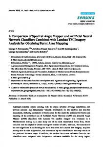
The derivation of SAM errors is due to the utilization of integral values of x and y instead of employing the deviations of pairs (x –x mean) and (y – y mean). Through an analysis of Table 4, it is possible to understand that the pairs of deviations (x –x mean) and (y – y mean) present opposite signs at negative correlation and equal signs at positive correlation. A visualization of this concept represented in a graph. Figure 1 graphs the mean deviations in the relationship between X and Y. The disposition of points through quadrants 2 and 3 indicates the presence of one positive correlation (Fig. 2a). However, the disposition of points in quadrants 1 and 4 indicates one negative correlation (Fig. 2b). Through the intermission of the deviation signs it is possible to detect the presence of positive or negative correlations. Thus, the employment of pair deviation inside of the SAM model provides a better estimate of the similarity degrees between X and Y. Table 4. Analysis of Pairs of Deviations Relative to the Mean During an Event of Positive and Negative Correlation Positive Correlation x 1 2 3 4 5
y 2 4 6 8 10
x-xm -2 -1 0 1 2
y-ym -4 -2 0 2 4
(x-xm)(y-ym) 8 2 0 2 8
Negative Correlation x 1 2 3 4 5
y 12 10 6 4 2
x-xm y-ym -2 4 -1 2 0 0 1 -2 2 -4
(x-xm)(y-ym) -8 -2 0 -2 -8
Figure 1 – Graphic area in relation to the deviations beginning at x mean and y mean.
Figure 2 – Exemplification of correlation: a) positive – with the major part of points presenting signals similar in relation at x mean and y mean; b) negative – with the major part of points with apposite signals in relation at x mean and y mean. Due to the SAM limitations described above, when compared with other methods it has demonstrated poor performances. Thus, Crósta et al. (1996, 1998) have had better results on the detection of targets using Tricorder instead of SAM in the area of Bodie, California. Also, Dickerhof et al. (1998) working with SAM obtained worse results when compared to Spectral Mixture Analysis (SMA) used for mineralogical identification and lithological mapping at Naxos Island, in Greece. 5
THE SPECTRAL METHOD SPECTRAL CORRELATION MAPPER (SCM) PROPOSITION
The Spectral Correlation Mapper (SCM) method is a derivative of Pearsonian Correlation Coefficient that eliminates negative correlation and maintains the SAM characteristic of minimizing the shading effect resulting in better results. The SCM varies from –1 to 1 and cos (SAM) varies from 0 to 1.
The SCM algorithm method, similar to SAM, uses the reference spectrum defined by the investigator, in accordance with the image s/he wants to classify. The algorithm was developed from IDL language and implemented as an application of the ENVI program. 6
THE SCM TEST FOR A REGION OF THE NIQUELÂNDIA MINE, BRAZIL
The SCM program was tested in the Niquelândia mine, for kaolinite features. With the objective of forming comparisons, the cos (SAM) calculation was performed, which presents the same value graduation as SCM. Both present as higher values the points of higher correlation. For kaolinite analysis, the spectrum interval is from 2.10730µm to 2. 27620µm which corresponds as bands 184 to 201 from the AVIRIS sensor. Such methods present better results when the calculation is accomplished inside the limits of the features at diagnostic absorption on mineral analysis. Figure 3 shows the images relatives to the treatment of cos (SAM) and SCM. Each image is accompanied by its respective entrance histograms and its output. Note that the SCM image presents a more accentuated contrast for the area with kaolinite (white regions) than is observed in the cos (SAM) image. The SCM histogram demonstrates that the major part of the pixels present negative correlation. Thus, the rich kaolinite areas are distinguished because they are of high intensity. However, the cos (SAM) does not obtain the same results due to the fact that it equally takes into account the positive and negative feature correlations. So, the cos (SAM) presents a very restricted variation from 0,9902 to 1 while SCM presents a wide variation of data from –85 to 1. The SCM can also be expressed in angles. Thus, negative correlation values must be transformed to zero applying the arcos (SCM) function (Fig. 4). To generate an image that emphasizes those dubious points, a subtraction operation was done between the cos (SAM) image and SCM In order to do so, a normalization of the images was done to make them compatible. This normalization was done through mean subtraction divided by standard deviation. As a result, we have an image where higher pixel values represent the places of the erroneous determination of the SAM method (Fig. 5). The visualization of profiles throughout the image-subtraction allows the emphasizing, by relative intensity, of the places where a divergent behavior between the two methods exists. Figure 5 presents the image profile through the imagesubtraction for one horizontal transect. On the analogous image form, the positive predominant pixels represent the pixels where the methods are divergent. The more prominent point of this profile is demonstrated by the spectral curve in comparison with the kaolinite (Fig. 6). Observe that a significant similarity exists between the kaolinite absorption bands and the emission of the pixel spectrum bands. 7
CONCLUSION
The SCM method implemented in SAM method allows for the detection of figures with negative correlation and presents better results for elimination of shading effect. The principal change of the proposal is on the utilization of pair deviations, which is different from the original SAM formulation.
SAM
Cos (SAM)
Figure 3 – Images relative to mineral identification of kaolinite according to the cos (SAM) and SCM.
Figure 4 – arcos (SCM+).
Figure 5 – Horizontal profile of image subtraction enhance difference between cos (SAM) and SCM.
Figure 6 – Comparison of spectral behavior of the anomalous pixel of the profile in relation to the kaolinite used as reference a) pixel curve, b) kaolinite curve, and c) superposition of two curves. ACKNOWLEDGEMENTS
The Brazilian Army has supported this work. We also thank Dr. Mírian Trindade Garret for her review and suggestions.
REFERENCES Bogliolo M.P, Teggi S., Buongiorno M.F, Pugnaghi S., 1998, Retrieving Ground Reflectance from MIVIS Data: A Case Study on Vulcano Island (Italy), 1st EARSeL Workshop on Imaging Spectroscopy, Remote Sensing Laboratories, University of Zurich, Switzerland, pp. 403-416. Boardman, 1992, SIPS User’s Guide Spectral Image Processing System, Version 1.2, Center for the Study of Earth from Space, Boulder, CO. 88 pp. Conel, James E; Hoover, G; Nolin, A; Alley, R; Margolis, J., 1992. Emperical Relationships Among SemiArid Landscape Endmembers Using the Spectral Angle Mapper (SAM) Algorithm, Summaries of the 4nd Annual JPL Airborne Geoscience Workshop, JPL Pub-92-14, AVIRIS Workshop. Jet Propulsion Laboratory, Pasadena, CA, pp. 150-151. Crósta, A. C., Sabine, C., Taranik, J. V., 1996, A Comparison of image processing methods for alteration mapping at Bodie, California, using 1992 AVIRIS data. Summaries of the Sixth JPL Airborne Earth Science Workshop, JPL Publication 96-1 v.1. Crósta, A. P.; Sabine, C. & Taranik J. V., 1998, Hydrothermal alteration mapping at Bodie, California, using AVIRIS Hyperpectral Data, Remote Sens. Environ 65:309-319 Dickerhof, C., Echtler, H., Kaufmann, H., Berger, M., Schlaepfer, M., Schaepman, M., Itten, K. & Doutsos, T., 1988, Mineral identification and lithological mapping on the island of Naxos (Greece) using DAIS 1915 hyperspectral data. 1st EARSeL Workshop on Imaging Spectroscopy, Remote Sensing Laboratories, University of Zurich, Switzerland, pp. 357-363. Kruse, F., A., Lefkoff, B., & Dietz, J. B., 1993, Expert System-Based Mineral Mapping in Northern Death Valley, California/Nevada, Using the Airborne Visible/Infrared Imaging Spectrometer (AVIRIS), Remote Sensing of Environment, vol.44, no.2, pp. 309-336. Kruse, FA; Lefkoff, A. B; Boardman, J. W.; Heiedbrecht; K. B. Shapiro, A. T.; Barloon, P. J.; Goetz, A. F. H., 1993, The Spectral Image Processing System (SIPS) – Interactive Visualization and Analysis of Imaging Spectrometer Data. REMOTE SENS. ENVIRON. 44:145-163. Kruse, F. A.; Lefkoff, A. B.; Boardman, J. W.; Heiedbrecht; Shapiro, A. T.; Barloon, P. J.; Goetz, A. F. H., 1992. The Spectral Image Processing System (SIPS) - Software for Integrated Analysis of AVIRIS Data Summaries of the 4th Annual JPL Airborne Geoscience Workshop, JPL Pub-92-14, AVIRIS Workshop. Jet Propulsion Laboratory, Pasadena, CA, pp. 23-25. McCubbin, I.; Lang, H., Green, R; Lang, H; Roberts, D, 1998, Mineral Mapping AVIRIS Data at Ray Mine AZ Summaries of the 7th JPL Airborne Earth Science Workshop, JPL Publication 97-21 v.1, pp. 269272. Riaza, Kaufmann, H, Zock, A, Müller, A, 1998, Mineral Mapping in Maktesh_Ramon (ISRAEL) Using DAIS 7915, 1st EARSeL Workshop on Imaging Spectroscopy, Remote Sensing Laboratories, University of Zurich, Switzerland, pp. 365-373. Richardson, L. L. & Kruse F. A., 1998, Identification and Classification of Mixed Phytoplankton Assemblages using AVIRIS image-derived Spectra, Summaries of the 8th JPL Airborne Earth Science Workshop. Yuhas, R. H; Goetz, AFH; Boardman, J. W., 1992. Discrimination Among Semi-Arid Landscape Endmembers Using Spectral Angle Mapper (SAM) Algorithm, Summaries of the 4th Annual JPL Airborne Geoscience Workshop, JPL Pub-92-14, AVIRIS Workshop. Jet Propulsion Laboratory, Pasadena, CA, pp. 147-150.