Speed Scaling Functions for Flow Time Scheduling based on Active ...

Speed Scaling Functions for Flow Time Scheduling based on Active Job Count Tak-Wah Lam1 , Lap-Kei Lee1 , Isaac K. K. To2 , and Prudence W. H. Wong2 1

Department of Computer Science, University of Hong Kong. {twlam, lklee}@cs.hku.hk 2 Department of Computer Science, University of Liverpool. {isaacto, pwong}@liverpool.ac.uk

Abstract. We study online scheduling to minimize flow time plus energy usage in the dynamic speed scaling model. We devise new speed scaling functions that depend on the number of active jobs, replacing the existing speed scaling functions in the literature that depend on the remaining work of active jobs. The new speed functions are more stable and also more efficient. They can support better job selection strategies to improve the competitive ratios of existing algorithms [5, 8], and, more importantly, to remove the requirement of extra speed. These functions further distinguish themselves from others as they can readily be used in the non-clairvoyant model (where the size of a job is only known when the job finishes). As a first step, we study the scheduling of batched jobs (i.e., jobs with the same release time) in the non-clairvoyant model and present the first competitive algorithm for minimizing flow time plus energy (as well as for weighted flow time plus energy); the performance is close to optimal.

1

Introduction

Energy usage is an important concern in recent research on online scheduling. A popular approach to reducing energy usage is dynamic speed scaling (see e.g., [10, 13]), which allows a processor to vary its speed dynamically. A processor incurs an energy of sα per unit time when running at speed s, where α ≥ 2 (typically 2 or 3 [10, 20]). Running a job slower saves energy, yet it takes longer and may affect performance. A lot of effort has been devoted to revisiting classical scheduling problems with dynamic speed scaling and energy concern taken into consideration (see [14] for a survey). The challenge arises from the conflicting objectives of providing good “quality of service” (QoS) and conserving energy. These studies first focused on the infinite speed model [24] where any speed may be used, and have recently shifted to the more realistic bounded speed model [12], which imposes a bound T on the maximum allowable speed. One commonly used QoS measure for job scheduling is the total flow time. Here, jobs with arbitrary size are released at unpredictable times and the flow ⋆

This research is partly supported by Hong Kong RGC Grant HKU/7140/06E and EPSRC Grant EP/E028276/1.

α=2 α=3 Infinite speed 5.236 [8] 7.940 [8] model (T = ∞) 2.667 [this paper] 3.252 [this paper] Bounded speed 10.472 with max speed 1.618T [5] 11.910 with max speed 1.466T [5] model 3.6 with max speed T [this paper] 4 with max speed T [this paper] Table 1. Results on clairvoyant scheduling for minimizing flow time plus energy. Note that the new results in this paper do not demand extra speed.

time of a job is the time elapsed since it arrives until it is completed. Preemption is allowed without penalty. When energy is not a concern, the objective is simply to minimize the total flow time of all jobs, and the online algorithm SRPT (shortest remaining processing time) is optimal [3]. If jobs carry weights, another online algorithm HDF (highest density first) has been shown to be (1 + 1/ǫ)competitive for weighted flow time, when using (1 + ǫ) times faster processor [9]; in fact, no online algorithm can be O(1)-competitive without extra speed [4]. The above results assume clairvoyance, i.e., the size of a job is known at release time. In some applications like operating systems, job size is only known when the job finishes. This is referred to as the non-clairvoyant model. The earlier work focused on batched jobs (i.e., all jobs have the same release time), and Motwani et al. [19] have shown that the online algorithm Round Robin is 2competitive for flow time. There is a matching lower bound of 2 when the number of jobs is large. Kim and Chwa [17] further showed that a weighted version of Round Robin is also 2-competitive for weighted flow time. For jobs with arbitrary release times, Kalyanasundaram and Pruhs [16] showed that SETF (shortest elapsed time first) is (1 + ǫ)-speed (1 + 1/ǫ)-competitive for flow time. The result has also been generalized to weighted flow time with the same performance [6,17]. Flow time and energy. To understand the tradeoff between flow time and energy, Albers and Fujiwara [1] proposed combining the dual objectives into a single objective of minimizing the sum of total flow time and energy. The intuition is that, from an economic viewpoint, users are willing to pay a certain (say, x) units of energy to reduce one unit of flow time. By changing the units of time and energy, one can further assume that x = 1 and thus would like to optimize total flow time plus energy. Albers and Fujiwara focused on the clairvoyant model and their work has been improved by Bansal et al. [5, 8]. As far as we know, there is no previous work on the non-clairvoyant model. In the infinite speed model, Bansal et al. [8] gave an O(1)-competitive online algorithm for minimizing flow time plus energy; precisely, the competitive ratio is µǫ γ1 , where ǫ is any positive constant, µǫ = max{(1 + 1/ǫ), (1 + ǫ)α } and 2(α−1) γ1 = max{2, α−(α−1) 1−1/(α−1) }. E.g., if α = 2, the competitive ratio is 5.236. Very recently, Bansal et al. [5] adapted this result to the bounded speed model. Assuming that the online algorithm can have a higher maximum speed of (1+ǫ)T for any ǫ > 0, the competitive ratio in this case increases slightly to µǫ γ2 , where γ2 = 2α/(α−(α−1)1−1/(α−1) ) = (2+o(1))α/ ln α. Table 1 shows the competitive ratios for some fixed α. Both results also hold for weighted flow time plus energy.

Follow-up questions. The speed function of the algorithms by Bansal et al. [5,8] depends on the remaining work of “active” jobs (i.e., jobs that have not been completed). There are several questions related to such a speed function.

– In the non-clairvoyant model, work-based speed functions are not applicable since job size, and hence remaining work, is not known to the online algorithm. Can one devise a speed function for the non-clairvoyant model? – Work-based speed functions would demand the processor speed to change continuously which is undesirable practically. Can one design a more stable speed function that changes in a discrete manner? – The algorithms in [5, 8] require extra speed even in the unweighted setting. In contrast, the classical result on flow-time scheduling does not need extra speed [3]. This is perhaps due to the inefficiency of the work-based speed functions; specifically, they are sometimes slower than a critical threshold n 1/α (( α−1 ) where n is the number of active jobs). When this happens, we can decrease the flow time plus energy by increasing the speed. It is natural to ask whether a speed function that never goes below this threshold can work without extra speed and gives a better competitive ratio. Our contribution. In this paper, we answer affirmatively the above questions by introducing new speed functions that depend on the number of active jobs. They are more stable, changing only at job arrival or completion. Using these functions leads to improvements in the clairvoyant model and provides the first competitive results on non-clairvoyant scheduling of batched jobs.

– Clairvoyant scheduling: Define the speed function AJC to be n1/α , where n is the number of active jobs. We use SRPT (instead of SJF (shortest job first) in [5,8]) to select jobs. Our algorithm is more competitive for minimizing flow time plus energy and does not need extra speed: for the infinite and bounded α−1 speed model, the competitive ratios are respectively β1 = 2/(1 − αα/(α−1) ) α−1 and β2 = 2(α + 1)/(α − (α+1)1/(α−1) ). Table 1 compares these ratios with those in [5, 8]. The improvement is more significant for large α, as β1 and β2 tend to 2α/ ln α, while µǫ γ1 and µǫ γ2 [5, 8] tend to 2(α/ ln α)2 . – Non-clairvoyant scheduling: We focus on batched jobs, i.e., when all jobs are released at time 0. For scheduling unweighted jobs, we use the speed n 1/α ) , where n is the total number of active jobs. function AJC∗ = ( α−1 Coupling with Round Robin, we give an algorithm that is (2− α1 )-competitive in the infinite speed model and 2-competitive in the bounded speed model. The latter inherits a lower bound of 2 from flow-time scheduling [19]. We can further generalize this algorithm for minimizing weighted flow time plus energy, and the corresponding ratios become (2 − α1 )2 and 4, respectively. Technically speaking, the analysis of existing clairvoyant algorithms requires indirect comparison via a notion called fractional flow. In contrast, we divide the time into “stable intervals”, and directly compare the flow time of the online algorithm against an optimal offline algorithm in each interval. This makes

the analysis tighter. For the non-clairvoyant algorithms, we first prove that the performance of our algorithm is close to that of a clairvoyant algorithm based on SJF (shortest job first) plus AJC∗ . Then we show that SJF-AJC∗ is optimal against any offline algorithm for minimizing flow time plus energy. Remarks. The theoretical study of energy-efficient scheduling was initiated by Yao, Demers and Shenker [24]. They considered deadline scheduling in the infinite speed model. Their result was improved by Bansal et al. [7], and extended to the bounded speed model by Chan et al. [12] and Bansal et al. [5]. Irani et al. [15] considered a setting where the processor has a sleep state. Pruhs et al. [21] also studied offline scheduling for minimizing the total flow time on a processor with a given amount of energy. The offline problem of minimizing the makespan subject to a fixed amount of energy has been studied in [11, 22]. Recently, multiprocessor setting has received attention, with interesting offline [11, 22] and online results [2, 18]. As some of these multiprocessor algorithms (in particular, [18]) are based on the single-processor algorithms in [5,8], our new result on clairvoyant scheduling immediately leads to an improvement.

2

Definitions and Notations

We consider a job set J to be scheduled on a processor whose speed can be varied between 0 and T , the speed bound. In the infinite speed model, T = ∞, so any speed is allowed. When running at speed s, the processor processes s units of work and consumes sα units of energy in each unit of time, where α ≥ 2. Preemption is allowed; a preempted job can resume at the point of preemption. We use ri and pi to denote the release time and work requirement (or size) of a job Ji in J , respectively. If ri = 0 for all jobs, we call J batched jobs. Consider a particular time t in a schedule of J . For any job Ji in J , we let qi denote its remaining work at t, and say it is active if ri ≤ t and qi > 0. The flow time Fi of Ji is the time elapsed it is completed. P since it arrives untilR ∞ The total flow time is given by F = i Fi . Note that F = 0 n(t) dt, where n(t) denotes the number of active jobs at time t, and the energy consumption is R∞ E = 0 s(t)α dt, where s(t) is the speed of the processor at time t. Our aim is to minimize the total flow time plus energy, G = F + E. We observe that each of E, F and G is the integration over all time from 0 to ∞. We call the integration over a period of time to be the contribution to their Rrespective value during that t period. E.g., the contribution to G from t1 to t2 is t12(n(t) + s(t)α ) dt.

3

Clairvoyant Scheduling with Arbitrary Release Times

In this section, we study the case where a job arrives at arbitrary time and its size is known upon arrival. Define the speed function AJC (active job count) to be min{T, n1/α }, where n is the number of active jobs and T is maximum speed. Coupling with SRPT, we have the algorithm SRPT-AJC. We first explain that SRPT gives the best job selection (Lemma 1). In the next two subsections, we analyze SRPT-AJC in the infinite speed and bounded speed models.

Lemma 1. Consider a job sequence J . Suppose a schedule S for J uses speed function f . Then, among all schedules of J using the speed function f , the one selecting jobs in accordance with SRPT incurs the least total flow time. Proof. We modify S in multiple steps to a SRPT schedule. In each step the new schedule S ′ has total flow time reduced. Then the lemma follows. Let t be the first time when S does not follow SRPT, running Ji instead of the shortest remaining work job Jj . S ′ differs from S during the time intervals since t when S runs either job: Jj is run to completion before Ji , using the same speed function. Jj thus completes in S ′ earlier than Ji does in S. So the sum of their completion time, and thus the total flow time, is less in S ′ than in S. ⊓ ⊔ 3.1

Analysis of SRPT-AJC for the Infinite Speed Model

We analyze SRPT-AJC for the infinite speed model, comparing it against an optimal offline schedule OPT. By Lemma 1, OPT uses the SRPT policy as well. Overview. Consider any time t. Let Ga (t) and Go (t) be the flow time plus energy incurred up to t by SRPT-AJC and OPT, respectively. We drop the parameter t when it refers to the current time. Our analysis exploits amortization and potential functions (e.g., [8, 12]): if there is a potential function Φ(t) and a value β such that the followings hold, then SRPT-AJC is β-competitive. – Boundary condition: Φ is initially 0 and finally non-negative. – Arrival condition: When a job is released, Φ does not increase. – Running condition: At any other time, the rate of change of Ga plus that dGo dΦ a of Φ is no more than β times the rate of change of Go , i.e., dG dt + dt ≤ β dt . We first show such a potential function Φ, whose design is motivated by the α−1 ). Then we show that the work in [5, 8]. We will choose β to be 2/(1 − αα/(α−1) above conditions hold, and thus can conclude the competitiveness of SRPT-AJC. Theorem 1. SRPT-AJC is β1 -competitive for flow time plus energy in the inα−1 ). finite speed model, where β1 = 2/(1 − αα/(α−1) Potential function Φ(t). Consider any time t. For any q ≥ 0, let na (q) denote the current number of active jobs with remaining work at least q in SRPT-AJC, and similarly no (q) for OPT. So na (0) and no (0) are the total number of active jobs in the schedules, which we abbreviate as na and no , respectively. It is useful to consider na (q) and no (q) as functions of q which change when a job arrives or runs for a while (see Fig. 3.1). We define the potential function as

Φ(t) = η

Z

0

∞

φ(q) dq , where φ(q) =

nX a (q) i=1

i1−1/α



− na (q)1−1/α no (q) ,

1−1/α α−1 and η = 2/(1 − αα/(α−1) ). (In bounded speed model, η = 2/(1 − (α+1) 1/(α−1) ).) At t = 0 or ∞, no job remains, so Φ = 0. The integration of the first term of φ(q) is proportional to the total flow time plus energy of SRPT-AJC after t if R ∞ Pna (q) 1−1/α no more job arrives (which is 2 0 dq), paying the cost once OPT i=1 i completes all jobs. The second term of φ(q) makes the arrival condition hold.

n(q)

n(q)

n(q)

q

(a)

(b)

q

(c)

p

q

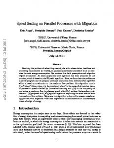
Fig. 1. (a) At any time, na (q) or no (q) (denoted by n(q) above) is a step function containing unit height stripes, the area under n(q) is the total remaining work. (b) If we run a job selected with SRPT at speed s for a period of time ∆, the top stripe shrinks by s∆. (c) When a job of size p is released, n(q) increases by 1 for all q ≤ p.

Lemma 2. When a job arrives, the change of Φ is non-positive. Proof. Suppose a job Jj arrives. For q > pj , na (q) and no (q), and hence φ(q), are unchanged. For q ≤ pj , both na (q) and no (q) increase by 1 (see Fig. 3.1(c)). So the first term of φ(q) increases by (na (q) + 1)1−1/α . The increase of the term na (q)1−1/α no (q) is interpreted in two-steps: (i) increase to (na (q)+1)1−1/α no (q), and (ii) increase to (na (q)+ 1)1−1/α (no (q)+ 1). The increase in step (ii), (na (q)+ 1)1−1/α , covers the increase in the first term of φ(q), so φ(q) cannot increase. ⊓ ⊔ Running condition. The rest of this section proves the following lemma.

Lemma 3. When no job arrives,

dGa dΦ dt + dt

α−1 o ≤ β1 dG dt where β1 = 2/(1− αα/(α−1) ).

Consider any time t. Let sa and so be the speed of SRPT-AJC and OPT, respectively, and qa and qo be the remaining work of the job they run. We divide the time line into stable intervals by breaking it when the following events occur. – – – –

A job arrives, or is completed by either SRPT-AJC or OPT. The speed sa or the job chosen by SRPT-AJC changes. The speed so or the job chosen by OPT changes. Either no (qa ) or na (qo ) changes.

Φ does not increase on job arrival (Lemma 2), and is unchanged on other events above (φ(q) changes for single q). So we focus on its change in a stable interval. We first bound dΦ dt . Consider a stable interval of length dt. We analyze dΦ as if φ(q) is modified in two steps: (i) na (q) decreases due to the execution of SRPT-AJC. (ii) no (q) decreases due to the execution of OPT. We denote these changes by dΦ1 and dΦ2 , respectively. Then dΦ = dΦ1 + dΦ2 . Lemma 4. Consider a stable interval of length dt. (i) dΦ1 ≤ η(no − na )dt; (ii) 1−1/α dΦ2 ≤ ηna so dt. Proof. (i) Consider SRPT-AJC. na (q) decreases from na to na − 1 for all q ∈ [qa − sa dt, qa ] (see Fig. 3.1(b)). For any q ∈ [qa − sa dt, qa ], φ(q) is changed by:   X nX na a −1 i1−1/α + na1−1/α no (q) i1−1/α − (na − 1)1−1/α no (q) − i=1

≤−

na1−1/α

+

n−1/α no (q) a

≤

i=1 1−1/α −na

no . + n−1/α a

(The first inequality is due to n1−1/α − (n − 1)1−1/α ≤ n−1/α for any n ≥ 1. The 1/α second holds since no (q) ≤ no .) Recall that sa = na . Integrating over all q, dΦ1 ≤ η(−na1−1/α + n−1/α no )(n1/α a a dt) = η(no − na )dt . (ii) Consider OPT. As in (i), φ(q) is changed only for q ∈ [qo − so dt, qo ]. Note that na (q) ≤ na for all q. Then for any q ∈ [qo − so dt, qo ], φ(q) is changed by −na (q)1−1/α (no (q) − 1) + na (q)1−1/α no (q) = na (q)1−1/α ≤ na1−1/α . 1−1/α

Integrating over all q, we have dΦ2 ≤ ηna

so dt.

⊓ ⊔

Proof (Lemma 3). We introduce a constant µ > 0 into Lemma 4 (ii) using the 1−1/α Young’s Inequality (see Corollary 9 of [8]), leading to dΦ2 ≤ ηna so dt ≤ α
ηs 1/α α a η(1 − α1 )µα/(α−1) na + αµoα dt . Since sa = na , dG = n + s = 2n . Also, a a a dt dGo α dt = no + so . Since dΦ = dΦ1 + dΦ2 , by Lemma 4 (i), we have  dGa dΦ 1
α/(α−1) sα  + ≤ 2na + η no − na + 1 − µ na + oα . dt dt α αµ Lemma 3 follows with β1 = η = 2/(1 − 3.2

α−1 ) αα/(α−1)

and µ = α−1/α .

(1) ⊓ ⊔

Analysis of SRPT-AJC for the Bounded Speed Model

We now turn to the bounded speed model. We use the same potential function 1−1/α while setting η = 2/(1− (α+1) 1/(α−1) ). Most of the analysis in Sect. 3.1 still holds, except Lemma 4 (i). As the speed used might be T instead of n1/α if n is large, the decrease in Φ1 is not sufficient to guarantee the original competitive ratio. We observe that the difference (na − no ) is upper bounded by T α (Lemma 5). Then the competitiveness is only slightly worse (Theorem 2). Lemma 5. At any time, the number of active jobs in SRPT-AJC and OPT satisfy na − no ≤ T α . Proof. This is trivial if na < T α . Suppose na ≥ T α at time t. Let t0 be the last moment before t when na changes from less than T α to at least T α . Consider the interval [t0 , t), where SRPT-AJC runs at full speed. Suppose k jobs arrive, and OPT completes x of them, so no ≥ k − x. Since SRPT maximizes the number of jobs completed at any time [23], SRPT-AJC also completes at least x jobs. So na increases by at most k − x ≤ no since t0 , and the lemma follows. ⊓ ⊔ Theorem 2. SRPT-AJC is β2 -competitive for flow time plus energy in the α−1 bounded speed model, where β2 = 2(α + 1)/(α − (α+1) 1/(α−1) ). Proof. The boundary and arrival conditions still hold. It remains to establish the running condition. Its analysis is split into two cases.

Case 1: na ≤ T α . The arguments in Sect. 3.1 still hold, leading to (1). Set 1−1/α µ = (α + 1)−1/α and recall that η = 2/(1 − (α+1) 1/(α−1) ), (1) implies

dGa dt

+ dΦ dt ≤

dGo ηno + (1 + 1/α)ηsα o ≤ β2 dt . α Case 2: na > T . The arguments in Sect. 3.1 hold, except Lemma 4 (i). We dGa α α o still have dG dt = no + so and dt = na + T < 2na . For dΦ1 ,

 T α 1/α dΦ1 ≤ η(−na1−1/α + n−1/α no )T dt = η(no − na ) dt . a na If no ≥ na , dΦ1 ≤ η(no − na )dt as before (since T α /na ≤ 1), leading to (1), so the arguments in Case 1 apply. If no < na , Lemma 5 implies  T α 1/α −η(na − no )1+1/α dΦ1 ≤ −η(na − no ) dt ≤ dt . 1/α na na Note that f (na − no ) ≥ f (na ) − f ′ (na ) no for the convex function f (x) = x1+1/α , 1+1/α 1/α which is equivalent to (na − no )1+1/α ≥ na − (1 + 1/α)na no . We thus have

1/α dt = η (1 + 1/α)no − na dt , dΦ1 ≤ −η (n1+1/α − (1 + 1/α)n1/α a a no )/na  sα  dΦ 1 1
α/(α−1) dGa µ na + oα . + ≤ 2na + η (1 + )no − na + 1 − and dt dt α α αµ Setting µ = (α + 1)−1/α , this implies

4

dGa dt

dGo 1 α + dΦ dt ≤ (1 + α )η(no + so ) = β2 dt .

⊓ ⊔

Non-clairvoyant Scheduling of Batched Jobs

In this section, we study non-clairvoyant scheduling of batched jobs. Recall that the online algorithm knows the size of a job only when the job finishes. AJC∗ and RR-AJC∗ . For batched jobs, we use a more energy-conservative n(t) 1/α ) }, where n(t) is the number of speed function AJC∗ , defined as min{T, ( α−1 active jobs at t. To cope with unknown job sizes, RR-AJC∗ uses AJC∗ with RR: split the processor equally among all active jobs. To analyze RR-AJC∗ , we consider a clairvoyant algorithm SJF-AJC∗ (shortest job first plus AJC∗ ). In Sect. 4.1, we show an interesting relation that the flow time plus energy incurred by RR-AJC∗ is close to that of SJF-AJC∗ . In Sect. 4.2 we complete the analysis by showing SJF-AJC∗ is optimal. In some applications, jobs may carry weights to reflect their importance. We use wi to denote the weight of a job Ji , and define its density ρi to be wi /pi . The weighted flow time of a job is simply its flow time multiplied by its weight. The above result can be generalized for weighted flow time plus energy as follows. AJW∗ and WRR-AJW∗ . The speed function AJW∗ (active job weight) is w(t) 1/α ) } where w(t) is the total weight of active jobs at t. defined as min{T, ( α−1 The algorithm WRR-AJW∗ uses AJW∗ with the WRR policy: split the processor among all active jobs in the ratio of their weights. We define the normalized work of a job as its work divided by its weight. Every active job has the same normalized processed work at any time.

To analyze WRR-AJW∗ , we consider a clairvoyant algorithm HDF-AJW∗ (highest density first plus AJW∗ ). The relation between WRR-AJW∗ and HDFAJW∗ is the same as before (Sect. 4.1). However, HDF-AJW∗ is not optimal. Yet we show that HDF-AJW∗ is competitive in Sect. 4.3. We use the weighted setting as a common platform, where RR-AJC∗ (resp. SJF-AJC∗ ) is WRR-AJW∗ (resp. HDF-AJW∗ ) with job weights all equal to one. Without loss of generality, we assume the input J = {J1 , J2 , . . . , Jn } is in increasing job density order, i.e., ρ1 ≤ ρ2 ≤ · · · ≤ ρn (ties are broken by job IDs). 4.1

Comparing WRR-AJW∗ against HDF-AJW∗

As jobs are batched, WRR impliesP that jobs complete in the order of normalized work, from Jn to J1 . Thus w(t) = ij=1 wj if Ji is the smallest normalized work job at t. We can thus compare WRR-AJW∗ against HDF-AJW∗ easily. Lemma 6. For scheduling batched jobs, the weighted flow time plus energy of WRR-AJW∗ is (i) at most (2 − 1/α) times of HDF-AJW∗ in the infinite speed model, and (ii) at most 2 times of HDF-AJW∗ in the bounded speed model. To prove Lemma 6, we focus on the contributions to weighted flow time and energy during the time when a particular job Ji is the job with the smallest normalized work in WRR-AJW∗ . Due to the WRR policy, each of the remaining jobs Jj with 1 ≤ j ≤ i is run for the same amount of normalized work. We thus evaluate the weighted flow time and energy incurred by WRR-AJW∗ during this period, denoted as Fw (Ji ) and Ew (Ji ). They are compared against the weighted flow time and energy incurred by HDF-AJW∗ to process that same amount of normalized work for each of these jobs, denoted as Fh (Ji ) and Eh (Ji ). We show that both Fw (Ji )/Fh (Ji ) and Ew (Ji )/Eh (Ji ) are no greater than (2 − 1/α) for T = ∞, and 2 for general T . Summing over all Ji leads to Lemma 6. Lemma 7. If T = ∞, Fw (Ji ) ≤ (2 − 1/α)Fh (Ji ) and Ew (Ji ) ≤ (2 − 1/α)Eh (Ji ). Proof. Due to the rules in the speed function AJW∗ , when T = ∞ we have Fw (Ji ) = (α − 1)Ew (Ji ) and Fh (Ji ) = (α − 1)Eh (Ji ). So it suffices to show Fw (Ji ) ≤ (2 − 1/α)Fh (Ji ). Let us first consider WRR-AJW∗ . Let ∆h be the normalized work processed P w(t) 1/α for each job J1 , . . . , Ji . We have seen that w(t) = ik=1 wk , s = ( α−1 ) . The amount of work processed for Jj (1 ≤ j ≤ i) is wj ∆h, so the total weighted flow Pi Pi Pi time incurred Fw (Ji ) = j=1 wj ∆h k=1 wk /s = (α−1)1/α ( j=1 wj )2−1/α ∆h. In contrast, HDF-AJW∗ runs only the highest density (i.e., least normalized Pj w(t) 1/α ) . The work) job. At time t when processing Jj , w(t) = k=1 wk , s = ( α−1 weighted flow time incurred for processing an amount of work wj ∆h for Jj is Pj Pj thus wj ∆h( k=1 wk )/s = (α − 1)1/α ∆h( k=1 wk )1−1/α wj . We thus have Fh (Ji ) = (α − 1)1/α ∆h

j i X X

j=1 k=1

wk

1−1/α

wj .


1−1/α Pi Pj To approximate j=1 wj , we use the staircase-like function k=1 wk Pj P Pj f (x) = ( k=1 wk )1−1/α if x ∈ [ j−1 k=1 wk , k=1 wk ) where 1 ≤ j ≤ i .

R Pij=1 wj Pj 1−1/α ( w ) w is exactly f (x) dx. On the other k j 0 j=1 k=1 Pi 1−1/α hand, f (x) ≥ x for all x ∈ [0, j=1 wj ). We thus have Pi Z Pij=1 wj j i X 1−1/α X ( j=1 wj )2−1/α 1−1/α x dx = , wj ≥ wk 2 − 1/α 0 j=1

Note that

Pi

k=1

and Fh (Ji ) ≥ (α − 1)1/α ∆h

Pi

j=1

wj


2−1/α

/(2 − α1 ) = Fw (Ji )/(2 − α1 ).

⊓ ⊔

Proof (Lemma 6). We obtain (i) (T = ∞) by summing the relations about Fh and Fw and those about Eh and Ew in Lemma 7 over all Ji . For (ii) (T < ∞), suppose WRR-AJW∗ processes ∆h normalized work for P each of J1 , . . . , Ji . We first focus on Ew (Ji ) and Eh (Ji ). If ( ij=1 wj /(α − 1))1/α ≤ T , Lemma 7 applies, so Ew (Ji ) ≤ (2 − 1/α)Eh (Ji ). Otherwise, we try to find a P k ∈ {1, . . . , i} such that kj=1 wj is exactly (α − 1)T α (so that the speed bound is just not exceeded). If no such k exists, for the sake of analysis we split some job Ju P into two jobs Ju1 and Ju2 with the same density and total weight, so that u−1 wu1 + j=1 wj = (α − 1)T α . We set k = u1. This job splitting does not affect the speed function, and thus the energy consumption, of either WRR-AJW∗ and HDF-AJW∗ (speed used for Ju1 , Ju2 and Ju are all T ). We now notice that both WRR-AJW∗ and HDF-AJW∗ run Jk+1 , . . . , Ji at speed T , consuming the same energy E0 . The other jobs are run as if T = ∞, so Lemma 7 leads to Ew (Ji ) − E0 ≤ (2 − 1/α)(Eh (Ji ) − E0 ). This implies Ew (Ji ) ≤ (2 − 1/α)Eh (Ji ). We now compare Fw (Ji ) and Fh (Ji ). Again the interesting case is when Pi ( j=1 wj /(α−1))1/α > T , otherwise Fw (Ji ) ≤ (2−1/α)Fh (Ji ) by Lemma 7. For Pi WRR-AJW∗ , the processor uses speed T , so the time needed is j=1 wj ∆h/T , Pi and Fw (Ji ) = ( j=1 wj )2 ∆h/T . For HDF-AJW∗ , the time needed to run Jj for wj ∆h units of work is at least wj ∆h/T (since the speed used cannot be faster P than T ), incurring weighted flow time of at least jk=1 wk wj ∆h/T . We thus Pi Pj Pi have Fh (Ji ) ≥ j=1 k=1 wk wj ∆h/T > ( j=1 wj )2 ∆h/2T = Fw (Ji )/2. Summing these relations over all Ji gives the desired ratio in Lemma 6. ⊓ ⊔ 4.2

Analysis of SJF-AJC∗

We show that the speed function AJC∗ minimizes the flow time plus energy for scheduling batched jobs using SJF (equivalently, SRPT) (Lemma 8), implying the optimality of SJF-AJC∗ for flow time plus energy. Combining with Lemma 6, we obtain the competitive ratio of RR-AJC∗ (Theorem 3). Lemma 8. Consider a set of batched jobs J . Among all schedules of J using SJF for job selection, the schedule that incurs the minimum flow time plus energy n(t) 1/α sets the speed at any time t as min{T, ( α−1 ) }, where n(t) is the number of active jobs at t.

Proof. Consider a particular job Ji in the optimal schedule. We only need to consider cases where its speed is constant, otherwise we can average the speed to reduce energy usage without affecting flow time. Note that n(t) is unchanged when Ji is run. Suppose Ji runs at speed s. Then its contribution to flow time n(t) 1/α plus energy is n(t)pi /s + sα−1 pi , which is minimized when s = ( α−1 ) . ⊓ ⊔ Theorem 3. For scheduling batched jobs to minimize flow time plus energy, the algorithm RR-AJC∗ is (i) (2 − 1/α)-competitive in the infinite speed model, and (ii) 2-competitive in the bounded speed model. Proof. Since every other schedule can be modified to the SJF-AJC∗ schedule by Lemma 1 and then Lemma 8 while reducing total flow time plus energy, SJF-AJC∗ is optimal for total flow time plus energy. The theorem thus follows naturally from Lemma 6. ⊓ ⊔ 4.3

Analysis of HDF-AJW∗

When jobs are weighted, the clairvoyant algorithm HDF-AJW∗ is not optimal for weighted flow time plus energy. Instead we analyze HDF-AJW∗ via a variant concerning fractional flow. Due to space limitation, we only sketch the ideas. Consider a schedule of J . At any time t, the fractional weight w bi of Ji is defined to be wi (qi /pi ) (recall that qi is the remaining work of Ji ). We define R∞ P bi . The fractional flow is defined as Fb = 0 w(t) b dt. We now w(t) b = Ji is active w define our variant of HDF-AJW∗ . Algorithm HDF-FW. It differs from HDF-AJW∗ only in the speed function, w(t) b which uses the speed function FW defined as ( α−1 )1/α at any time t. We follow the framework in Sect. 4.2 to show the optimality of HDF-FW: Firstly, HDF minimizes fractional flow for a fixed speed function. Secondly, FW minimizes the fractional flow plus energy for scheduling batched jobs using HDF. Lemma 9. Consider a set of weighted batched jobs. The algorithm HDF-FW is optimal for minimizing the fractional flow plus energy of the schedule. By comparing the contribution to the weighted flow time plus energy of HDF-AJW∗ against that to the fractional flow plus energy of HDF-FW when each job Ji is running, we can show the following lemma. bhf be the fractional flow plus Lemma 10. Consider a set of batched jobs. Let G energy with HDF-FW. Then the weighted flow time plus energy with HDF-AJW∗ b hf in the infinite speed model, and (ii) Gh ≤ 2G b hf in the is (i) Gh ≤ (2 − 1/α)G bounded speed model. We note that for any schedule, the fractional flow is at most the weighted flow time. Thus HDF-AJW∗ is (2 − 1/α)-competitive for weighted flow time plus energy. Together with Lemma 6, we obtain the competitive ratio of WRR-AJW∗ . Theorem 4. Consider a set of weighted batched jobs. The algorithm WRR-AJW∗ is (i) (2 − 1/α)2 -competitive in the infinite speed model, and (ii) 4-competitive in the bounded speed model.

References 1. S. Albers and H. Fujiwara. Energy-efficient algorithms for flow time minimization. ACM Trans. Alg., 3(4):49, 2007. 2. S. Albers, F. Muller, and S. Schmelzer. Speed scaling on parallel processors. In Proc. SPAA, pages 289–298, 2007. 3. K. R. Baker. Introduction to Sequencing and Scheduling. Wiley, New York, 1974. 4. N. Bansal and H. L. Chan. Weighted flow time does not have O(1) competitive algorithms. Manuscript. 5. N. Bansal, H. L. Chan, T. W. Lam, and L. K. Lee. Scheduling for speed bounded processors. In Proc. ICALP, 2008. To appear. 6. N. Bansal and K. Dhamdhere. Minimizing weighted flow time. ACM Trans. Alg., 3(4):39, 2007. 7. N. Bansal, T. Kimbrel, and K. Pruhs. Speed scaling to manage energy and temperature. J. ACM, 54(1), 2007. 8. N. Bansal, K. Pruhs, and C. Stein. Speed scaling for weighted flow time. In Proc. SODA, pages 805–813, 2007. 9. L. Becchetti, S. Leonardi, A. Marchetti-Spaccamela, and K. Pruhs. Online weighted flow time and deadline scheduling. J. Discrete Algorithms, 4(3):339–352, 2006. 10. D. Brooks, P. Bose, S. Schuster, H. M. Jacobson, P. Kudva, A. Buyuktosunoglu, J.-D. Wellman, V. V. Zyuban, M. Gupta, and P. W. Cook. Power-aware microarchitecture: Design and modeling challenges for next-generation microprocessors. IEEE Micro, 20(6):26–44, 2000. 11. D. P. Bunde. Power-aware scheduling for makespan and flow. In Proc. SPAA, pages 190–196, 2006. 12. H. L. Chan, W. T. Chan, T. W. Lam, L. K. Lee, K. S. Mak, and P. W. H. Wong. Energy efficient online deadline scheduling. In Proc. SODA, 2007. 13. D. Grunwald, P. Levis, C. B. Morrey, and M. Neufeld. Policies for dynamic clock scheduling. In Proc. OSDI, pages 73–86, 2000. 14. S. Irani and K. Pruhs. Algorithmic problems in power management. SIGACT News, 32(2):63–76, 2005. 15. S. Irani, S. Shukla, and R. Gupta. Algorithms for power savings. ACM Trans. Alg., 3(4):41, 2007. 16. B. Kalyanasundaram and K. Pruhs. Speed is as powerful as clairvoyance. J. ACM, 47(4):617–643, 2000. 17. J.-H. Kim and K.-Y. Chwa. Non-clairvoyant scheduling for weighted flow time. IPL, 87(1):31–37, 2003. 18. T. W. Lam, L. K. Lee, I. K. K. To, and P. W. H. Wong. Competitive non-migratory scheduling for flow time and energy. In Proc. SPAA, pages 256–264, 2008. 19. R. Motwani, S. Phillips, and E. Torng. Nonclairvoyant scheduling. Theoretical Computer Science, 130(1):17–47, 1994. 20. T. N. Mudge. Power: A first-class architectural design constraint. IEEE Comp., 34(4):52–58, 2001. 21. K. Pruhs, P. Uthaisombut, and G. Woeginger. Getting the best response for your erg. In Proc. SWAT, pages 14–25, 2004. 22. K. Pruhs, R. van Stee, and P. Uthaisombut. Speed scaling of tasks with precedence constraints. In Proc. WAOA, pages 307–319, 2005. 23. L. Schrage. A proof of the optimality of the shortest remaining processing time discipline. Operations Research, 16(3):687–690, 1968. 24. F. Yao, A. J. Demers, and S. Shenker. A scheduling model for reduced CPU energy. In Proc. FOCS, pages 374–382, 1995.