Spike-and-Slab Sparse Coding for Unsupervised Feature Discovery

Spike-and-Slab Sparse Coding for Unsupervised Feature Discovery

Ian J. Goodfellow, Aaron Courville, Yoshua Bengio D´epartement d’informatique et de recherche op´erationnelle Universit´e de Montr´eal Montr´eal, QC H3T 1J4 {goodfeli@iro.,courvila@iro.,yoshua.bengio@}umontreal.ca

Abstract We introduce spike-and-slab sparse coding (S3C), an unsupervised feature discovery algorithm. S3C is based on a generative model that resembles both the spike-and-slab RBM and sparse coding. Since exact inference in this model is intractable, we derive a structured variational inference procedure and employ a variational EM training algorithm. We demonstrate that this approach improves upon the supervised learning capabilities of both sparse coding and the ssRBM on the CIFAR-10 dataset. We evaluate our approach’s potential for semi-supervised learning on subsets of CIFAR-10. We use our method to win the NIPS 2011 Workshop on Challenges In Learning Hierarchical Models’ Transfer Learning Challenge.

1

The S3C model

The S3C model consists of latent binary spike variables h ∈ {0, 1}N , latent real-valued slab variables s ∈ RN , and real-valued D-dimensional visible vector v ∈ RD generated according to this process: ∀i ∈ {1, . . . , N }, d ∈ {1, . . . , D}, −1 −1 p(hi = 1) = σ(bi ), p(si | hi ) = N (si | hi µi , αii ), p(vd | s, h) = N (vd | Wd: (h ◦ s), βdd )

(1)

where σ is the logistic sigmoid function, b is a set of biases on the spike variables, µ and W govern the linear dependence of s on h and v on s respectively, α and β are diagonal precision matrices of their respective conditionals, and h ◦ s denotes the element-wise product of h and s. To avoid overparameterizing the distribution, we constrain the columns of W to have unit norm, as in sparse coding. We restrict α to be a diagonal matrix and β to be a diagonal matrix or a scalar. We refer to the variables hi and si as jointly defining the ith hidden unit, so that there are are total of N rather than 2N hidden units. The state of a hidden unit is best understood as hi si , that is, the spike variables gate the slab variables. In the subsequent sections we describe how this model occupies a middle ground between sparse coding and the ssRBM, avoiding many disadvantages of both. Further related work is ommitted due to lack of space in this workshop application. 1.1

Comparison to sparse coding

Sparse coding has been widely used to discover features for classification (Raina et al., 2007). Recently Coates and Ng (2011a) showed that this approach achieves excellent performance on the CIFAR10 object recognition dataset. Sparse coding (Olshausen and Field, 1997) describes a class of generative models where the observed data v is normally distributed given a set of continuous latent variables s and a dictionary matrix W : v ∼ N (W s, σI). Sparse coding places a factorial prior on s such as a Cauchy or Laplace distribution, chosen to encourage the posterior mode of p(s | v) to be sparse. One can derive the S3C model from sparse coding by replacing the factorial Cauchy or Laplace prior with a spike-and-slab prior. 1

One drawback of sparse coding is that the latent variables are not merely encouraged to be sparse; they are encouraged to remain close to 0, even when they are active. This kind of regularization is not necessarily undesirable, but in the case of simple but popular priors such as the Laplace prior (corresponding to an L1 penalty on the latent variables s), the degree of regularization on active units is confounded with the degree of sparsity. There is little reason to believe that in realistic settings, these two types of complexity control should be so tightly bound together. The S3C model avoids this issue by controlling the sparsity of units via the b parameter that determines how likely each spike unit is to be active, while separately controlling the magnitude of active uits via the µ and α parameters that govern the distribution over s. Sparse coding has no parameter analogous to µ and cannot control these aspects of the posterior independently. Sparse coding is also difficult to integrate into a deep generative model of data such as natural images. While Yu et al. (2011) and Zeiler et al. (2011) have recently shown some success at learning hierarchical sparse coding, our goal is to integrate the feature extraction scheme into a proven generative model framework such as the deep Boltzmann Machine (Salakhutdinov and Hinton, 2009). Existing inference schemes known to work well in the DBM-type setting are all either sample-based or are based on variational approximations to the model posteriors, while sparse coding schemes typically employ MAP inference. Our use of variational inference makes the S3C framework well suited to integrate into the known successful strategies for learning and inference in DBM models. It is not obvious how one can employ a variational inference strategy to standard sparse coding with the goal of achieving sparse feature encoding. 1.2

Comparison to Restricted Boltzmann Machines

The S3C model also resembles another class of models commonly used for feature discovery: the RBM. An RBM (Smolensky, 1986) is an energy-based model defined through an energy function that describes the interactions between the obversed data variables and a set of latent variables. It is possible to interpret the S3C as an energy-based model, by rearranging p(v, s, h) to take the form exp{−E(v, s, h)}/Z, with the following energy function: 1 E(v, s, h) = 2

!T v−

X

Wi si hi

! β

v−

i

X

Wi si hi

i

+

N N X 1X αi (si − µi hi )2 − bi hi , 2 i=1 i=1

(2)

The ssRBM model family is a good starting point for S3C because it has demonstrated both reasonable performance as a feature discovery scheme and remarkable performance as a generative model (Courville et al., 2011). Within the ssRBM family, S3C’s closest relative is a variant of the µ-ssRBM, defined by the following energy function: E(v, s, h) = −

N X i=1

v T βWi si hi +

N N X 1 T 1X b i hi , αi (si − µi hi )2 − v βv + 2 2 i=1 i=1

(3)

where the variables and parameters are defined identically to the S3C. Comparison of equations 2 and 3 reveals that the simple addition of a latent factor interaction term 12 (h ◦ s)T W T βW (h ◦ s) to the ssRBM energy function turns the ssRBM into the S3C model. With the inclusion of this term S3C moves from an undirected ssRBM model to the directed graphical model, described in equation (1). This change from undirected modeling to directed modeling has three important effects, that we describe in the following sections. The effect on the partition function: The most immediate consequence of the transition to directed modeling is that the partition function becomes tractable. This changes the nature of learning algorithms that can be applied to the model, since most of the difficulty in training an RBM comes from estimating the gradient of the log partition function. The partition function of S3C is also guaranteed to exist for all possible settings of the model parameters, which is not true of the ssRBM. The effect on the posterior: RBMs have a factorial posterior, but S3C and sparse coding have a complicated posterior due ot the “explaining away” effect. This means that for RBMs, features defined by similar basis functions will have similar activations, while in directed models, similar features will compete so that only the most relevant feature will remain active. As shown by Coates and Ng (2011a), the sparse Gaussian RBM is not a very good feature extractor – the set of basis functions W learned by the RBM actually work better for supervised learning when these parameters are plugged into a sparse coding model than when the RBM itself is used for feature extraction. We think this is due to the factorial posterior. In the vastly overcomplete setting, being able to selectively activate a small set of features likely provides S3C a major advantage in discriminative capability. 2

Distribution of [hi ]

106

0.016 0.015

Q [h]

104 103

Mean of

log number of occurrences

105

Sparsification during inference

0.014 0.013

102 0.012

101 1000.0

0.2

0.4

[hi ]

0.6

0.8

0.0110

1.0

5 15 10 Damped parallel fixed point updates

20

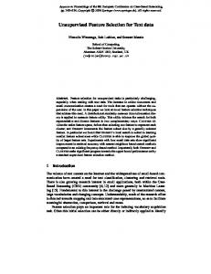
Figure 1: (Left) Q imposes a sparse distribution on h; Q(hi ) < .01 91.8% of the time. The samples in this histogram are values of Q(hi ) for 1600 different hidden units from a trained model applied to 100 different image patches. (Right) The inference procedure sparsifies the representation due to the explaining-away effect. Q is initialized at the prior, which is very sparse. The data then drives Q to become less sparse, but subsequent iterations make Q become sparse again.

The effect on the prior: The addition of the interaction term causes S3C to have a factorial prior. This probably makes it a poor generative model, but this is not a problem for the purpose of feature discovery.

2

Other related work

The notion of a spike-and-slab prior was established in statistics by Mitchell and Beauchamp (1988). Outside the context of unsupervised feature discovery for supervised, semi-supervised and selftaught learning, the basic form of the S3C model (i.e. a spike-and-slab latent factor model) has appeared a number of times in different domains (L¨ucke and Sheikh, 2011; Garrigues and Olshausen, 2008; Mohamed et al., 2011). To this literature, we contribute an inference scheme that scales to the kinds of object classifications tasks that we consider. We outline this inference scheme next.

3

Variational EM for S3C

Having explained why S3C is a powerful model for unsupervised feature discovery we turn to the problem of how to perform learning and inference in this model. Because computing the exact posterior distribution is intractable, we derive an efficient and effective inference mechanism and a variational EM learning algorithm. We turn to variational EM (Saul and Jordan, 1996) because this algorithm is well-suited for models with latent variables whose posterior is intractable. It works by maximizing a variational lower bound on the log-likelihood called the energy functional (Neal and Hinton, 1999). More specifically, it is a variant of the EM algorithm (Dempster et al., 1977) with the modification that in the E-step, we compute a variational approximation to the posterior rather than the posterior itself. While our model admits a closed-form solution to the M-step, we found that online learning with small gradient steps on the M-step objective worked better in practice. We therefore focus our presentation on the E-step, given in Algorithm 1. The goal of the variational E-step is to maximize the energy functional with respect to a distribution Q over the unobserved variables. We can do this by selecting the Q that minimizes the Kullback– Leibler divergence: DKL (Q(h, s)kP (h, s|v)) (4)

where Q(h, s) is drawn from a restricted family of distributions. This family can be chosen to ensure that Q is tractable. Our E-step can be seen as analogous to the encoding step of the sparse coding algorithm. The key difference is that while sparse coding approximates the true posterior with a MAP point estimate of 3

1400

Inference by Optimization

0.70

1600

Test Set Accuracy

Energy Functional

1500

1700 1800

0.65 0.60 0.55

1900 20000

CIFAR-10 Learning Curve

0.75

5 15 10 Damped parallel fixed point updates

0.500

20

SC S3C 200

400 600 800 Labeled Training Examples Per Class

1000

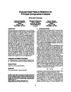
Figure 2: (Left) The energy functional of a batch of 5000 image patches increases during the E-step. (Right) Semi-supervised classification accuracy on CIFAR-10. In both cases the hyperparameters for the unsupervised stage were optimized for performance on the full CIFAR-10 dataset, not re-optimized for each point on the learning curve.

the latent variables, we approximate the true posterior with the distribution Q. We use the family Q(h, s) = Πi Q(hi , si ). Observing that eq. (4) is an instance of the Euler-Lagrange equation (Gelfand, 1963), we find that the solution must take the form ˆ i , Q(si | hi ) = N (si | hi sˆi , (αi + hi W T βWi )−1 ) Q(hi ) = h i

(5)

ˆ i and sˆi must be found by an iterative process. In a typical application of variational inwhere h ference, the iterative process consists of sequentially applying fixed point equations that give the ˆ i and sˆi for one factor Q(hi , si ) given the value all of the other optimal value of the parameters h factors’ parameters. This process is only guaranteed to decrease the KL divergence if applied to ˆ 1 and sˆ1 to optimize Q(h1 , s1 ), then updating h ˆ 2 and each factor sequentially, i.e. first updating h sˆ2 to optimize Q(h2 , s2 ), and so on. In a typical application of variational inference, the optimal values for each update are simply given by the solutions to the Euler-Lagrange equations. For S3C, we make three deviations from this standard approach. Because we apply S3C to very large-scale problems, sequential updates across all N factors require too much runtime. We instead update all of the factors in parallel, shrinking the update by a damping coefficient. This approach is not guaranteed to decrease the KL divergence on each iteration but is a widely applied approach that works well in practice (Koller and Friedman, 2009). In the case of S3C, the use of damped updates necessitates a second change from the standard ˆ i and sˆi are updated simultaneapproach to variational approximations. In the standard approach, h ously via the standard Euler-Lagrange solution. This simultaneous update means that the solution ˆ i assumes that sˆi will also reach its optimal value. The use of damping means that sˆi will not to h ˆ i . We find that this is very important reach its optimal value, and this invalidates the solution to h in practice, and that damping can cause the KL divergence to increase on each iteration, even if updating each factor sequentially. To resolve this problem, we use the joint solution only to derive the functional form of the eventual solution, eq. (5). We then solve ∂∂hˆ DKL = 0 and ∂∂sˆi DKL = 0 to i ˆ i is still optimal obtain a separate fixed point equation for each parameter. This way, the update for h even if the update to sˆi has been damped. One final deviation from the standard approach is necessary for S3C. We clip the update to sˆ so that if sˆnew has the opposite sign from sˆ, its magnitude is at most ρˆ s. In all of our experiments we used ρ = 0.5 but any value in [0, 1] is sensible. This prevents a case where two mutually inhibitory s units inhibit each other so strongly that rather than being driven to 0 both change sign and actually increase in magnitude. This case is a failure mode of the parallel updates that can result in sˆ amplifying without bound if clipping is not used. 4

We include some visualizations that demonstrate the effect of our E-step. Figure 1 (right) shows that it produces a sparse representation. Figure 1 (left) shows that the explaining-away effect incrementally makes the representation more sparse. Figure 2 (left) shows that the E-step increases the energy functional. Algorithm 1 Fixed-Point Inference ˆ (0) = σ(b) and s Initialize h ˆ(0) = µ. for k=0:K do Compute the individually optimal value s ˆ∗ hP i i for each i simultaneously: ˆ ˆ(k) µi αii + v T βWi − Wi β j6=i Wj hj s j ∗ s ˆi = αii + WiT βWi Clip reflections by assigning

∗

(k)

si for all i such that sign(ˆ s∗ i ) 6= sign(ˆ Damp the updates by assigning

(k)

si ) and |ˆ s∗ i | > ρ|ˆ

(k+1)

s ˆi

(k)

= ηc + (1 − η)ˆ s

where η ∈ (0, 1]. ˆ Compute the individually optimal values for0h: 0 ˆ ∗ = σ @@v − h i

(k+1) ˆ (k) hj

X

Wj s ˆj

j6=i

−

1 2

(k+1)

αii (ˆ si

(k)

ci = ρsign(ˆ si )|ˆ si | |, and assigning ci = s ˆ∗ i for all other i.

2

− µi ) −

1 2

−

1 2

1T (k+1) A

Wi s ˆi

T

(k+1)

βWi s ˆi

log(αii + Wi βWi ) +

1 2

+ bi

« log(αii )

ˆ Damp the update to h: ˆ (k+1) = η h ˆ ∗ + (1 − η)h ˆ (k) h end for

4

Results

We conducted experiments to evaluate the usefulness of S3C features for supervised learning and semi-supervised learning on the CIFAR-10 (Krizhevsky and Hinton, 2009) dataset, consisting of color images of animals and vehicles. It contains ten labeled classes, with 5000 train and 1000 test examples per class. For all experiments, we used the same procedure as Coates and Ng (2011a). CIFAR-10 consists of 32 × 32 images. We train our feature extractor on 6 × 6 contrast-normalized and ZCA-whitened patches from the training set. At test time, we extract features from all 6×6 patches on an image, then average-pool them. The average-pooling regions are arranged on a non-overlapping grid. Finally, we train a linear SVM on the pooled features. Coates and Ng (2011a) used 1600 basis vectors in all of their sparse coding experiments. They postprocessed the sparse coding feature vectors by splitting them into the positive and negative part for a total of 3200 features per average-pooling region. They average-pool on a 2 × 2 grid for a toal of 12,800 features per image. We used EQ [h] as our feature vector. This does not have a negative part, so using a 2 × 2 grid we would have only 6,400 features. In order to compare with similar sizes of feature vectors we used a 3 × 3 pooling grid for a total of 14,400 features. 4.1

CIFAR-10

On CIFAR-10, S3C achieves a test set accuracy of 78.3 ± 0.9 % with 95% confidence (or 76.2 ± 0.9 % when using a 2 × 2 grid). Coates and Ng (2011a) do not report test set accuracy for sparse coding with “natural encoding” (i.e., extracting features in a model whose parameters are all the same as in the model used for training) but sparse coding with different parameters for feature extraction than training achieves an accuracy of 78.8 ± 0.9% (Coates and Ng, 2011a). Since we have not enhanced our performance by modifying parameters at feature extraction time these results seem to indicate that S3C is roughly equivalent to sparse coding for this classification task. S3C also outperforms ssRBMs, which require 4,096 basis vectors per patch and a 3×3 pooling grid to achieve 76.7±0.9% accuracy. All of these approaches are close to the state of the art of 82.0 ± 0.8 %, which used a three layer network (Coates and Ng, 2011b). We also used CIFAR-10 to evaluate S3C’s semi-supervised learning performance by training the SVM on small subsets of the CIFAR-10 training set, but using features that were learned on the entire CIFAR-10 train set. The results, summarized in Figure 2 (right) show that S3C is most advantageous 5

for medium amounts of labeled data. S3C features thus include an aspect of flexible regularization– they improve generalization for smaller training sets yet do not cause underfitting on larger ones.

5

Transfer Learning Challenge

For the NIPS 2011 Workshop on Challenges in Learning Hierarchical Models (Le et al., 2011), the organizers proposed a transfer learning competition. This competition used a dataset consisting of 32 × 32 color images, including 100,000 unlabeled examples, 50,000 labeled examples of 100 object classes not present in the test set, and 120 labeled examples of 10 object classes present in the test set. The test set was not made public until after the competition. We chose to disregard the 50,000 labels and treat this as a semi-supervised learning task. We applied the same approach as on CIFAR-10 and won the competition, with a test set accuracy of 48.6 %.

6

Conclusion

We have motivated the use of the S3C model for unsupervised feature discovery. We have described a variational approximation scheme that makes it feasible to perform learning and inference in large-scale S3C models. Finally, we have demonstrated that S3C is an effective feature discovery algorithm for supervised, semi-supervised, and self-taught learning.

6

Acknowledgements This work was funded by DARPA and NSERC. The authors would like to thank Pascal Vincent for helpful discussions. The computation done for this work was conducted in part on computers of RESMIQ, Clumeq and SharcNet. We would like to thank the developers of theano (Bergstra et al., 2010) and pylearn2 (Warde-Farley et al., 2011).

References Bergstra, J., Breuleux, O., Bastien, F., Lamblin, P., Pascanu, R., Desjardins, G., Turian, J., Warde-Farley, D., and Bengio, Y. (2010). Theano: a CPU and GPU math expression compiler. In Proceedings of the Python for Scientific Computing Conference (SciPy). Oral Presentation. Coates, A. and Ng, A. Y. (2011a). The importance of encoding versus training with sparse coding and vector quantization. In ICML 28. Coates, A. and Ng, A. Y. (2011b). Selecting receptive fields in deep networks. In NIPS 2011. Courville, A., Bergstra, J., and Bengio, Y. (2011). Unsupervised models of images by spike-and-slab RBMs. In Proceedings of the Twenty-eight International Conference on Machine Learning (ICML’11). Dempster, A. P., Laird, N. M., and Rubin, D. B. (1977). Maximum-likelihood from incomplete data via the EM algorithm. Journal of Royal Statistical Society B, 39, 1–38. Garrigues, P. and Olshausen, B. (2008). Learning horizontal connections in a sparse coding model of natural images. In NIPS’07, pages 505–512. MIT Press, Cambridge, MA. Gelfand, I. M. (1963). Calculus of Variations. Dover. Koller, D. and Friedman, N. (2009). Probabilistic Graphical Models: Principles and Techniques. MIT Press. Krizhevsky, A. and Hinton, G. (2009). Learning multiple layers of features from tiny images. Technical report, University of Toronto. Le, Q. V., Ranzato, M., Salakhutdinov, R., Ng, A., and Tenenbaum, J. (2011). NIPS Workshop on Challenges in Learning Hierarchical Models: Transfer Learning and Optimization. https://sites.google.com/ site/nips2011workshop. L¨ucke, J. and Sheikh, A.-S. (2011). A closed-form EM algorithm for sparse coding. Mitchell, T. J. and Beauchamp, J. J. (1988). Bayesian variable selection in linear regression. J. Amer. Statistical Assoc., 83(404), 1023–1032. Mohamed, S., Heller, K., and Ghahramani, Z. (2011). Bayesian and l1 approaches to sparse unsupervised learning. Neal, R. and Hinton, G. (1999). A view of the em algorithm that justifies incremental, sparse, and other variants. In M. I. Jordan, editor, Learning in Graphical Models. MIT Press, Cambridge, MA. Olshausen, B. A. and Field, D. J. (1997). Sparse coding with an overcomplete basis set: a strategy employed by V1? Vision Research, 37, 3311–3325. Raina, R., Battle, A., Lee, H., Packer, B., and Ng, A. Y. (2007). Self-taught learning: transfer learning from unlabeled data. In Z. Ghahramani, editor, ICML 2007, pages 759–766. ACM. Salakhutdinov, R. and Hinton, G. (2009). Deep Boltzmann machines. In Proceedings of the Twelfth International Conference on Artificial Intelligence and Statistics (AISTATS 2009), volume 8. Saul, L. K. and Jordan, M. I. (1996). Exploiting tractable substructures in intractable networks. In NIPS’95. MIT Press, Cambridge, MA. Smolensky, P. (1986). Information processing in dynamical systems: Foundations of harmony theory. In D. E. Rumelhart and J. L. McClelland, editors, Parallel Distributed Processing, volume 1, chapter 6, pages 194–281. MIT Press, Cambridge. Warde-Farley, D., Goodfellow, I., Lamblin, P., Desjardins, G., Bastien, F., and Bengio, Y. (2011). pylearn2. http://deeplearning.net/software/pylearn2. Yu, K., Lin, Y., and Lafferty, J. (2011). Learning image representations from the pixel level via hierarchical sparse coding. In CVPR’11: IEEE Conference on Computer Vision and Pattern Recognition, pages 1713– 1720, Colorado Springs, CO. Zeiler, M., Taylor, G., and Fergus, R. (2011). Adaptive deconvolutional networks for mid and high level feature learning. In Proc. International Conference on Computer Vision (ICCV’11), pages 2146–2153. IEEE.

7