Split Point Selection and Recovery for Value Speculation ... - CiteSeerX

MICRO32 SUBMISSION

6/8/99 7:26:49 PM

Split Point Selection and Recovery for Value Speculation Scheduling Chao-ying Fu

Allan D. Knies∗

Thomas M. Conte

∗Intel Corporation Mail Stop SC12-304 2200 Mission College Blvd. Santa Clara, CA 95052 [email protected]

Department of Electrical and Computer Engineering North Carolina State University Raleigh, NC 27695-7911 {cfu, conte}@eos.ncsu.edu

Abstract This paper extends previous work in value speculation scheduling [14] with an expanded ISA, new recovery code generation methods, and better instruction selection techniques. Our results show that critical instructions are not as predictable as non-critical instructions, instructions at the top of local critical paths have higher predictability than instructions in the middle, and that long-latency instructions have lower predictability than one-cycle instructions. Results from various split point selection heuristics show that breaking true data dependencies of long-latency instructions on local critical paths provides larger cycle savings than only predicting top or middle instructions. This paper also provides empirical results showing the relationship between the predictability of instructions with their latency, location within a dependence chain, and criticality. We also analyze potential critical path reduction when a compiler is allowed to choose the best predictor on a per-instruction basis. Keywords: value speculation, value prediction, critical path reduction, instruction scheduling, instruction level parallelism.

1.

Introduction

Chains of true data dependencies are a significant limit to the amount of instruction level parallelism (ILP) that can be exploited by compilers and microprocessors. Many studies [1], [2], [7], [8], [14], [16], [17], [18], [19], [20] have shown value speculation to be a promising approach for overcoming this limitation. To date, most of the literature has focused on implicit parallel architectures with superscalar cores (except [14], [15], and [19] which concentrate on statically scheduled machines). This paper extends the initial work of value speculation scheduling (VSS) [14], and discusses techniques to deploy value speculation in a processor that uses an explicitly parallel instruction computing (EPIC) ISA. Our studies are based on the recently disclosed IA-64 architecture [22] with the addition of our own experimental instructions to support a wide variety of value prediction experiments. Since EPIC architectures and compilers are already capable of performing compiler-directed and hardware-managed optimizations to exploit more ILP

1

(such as control speculation [21], [22] and data speculation [9], [22]), VSS techniques and the value prediction instruction set architecture are easy to incorporate into existing infrastructure. The effectiveness of a value speculation technique relies not only on the predictability of instructions, but also the potential speedup from predicting those instructions. Many value predictor designs have been proposed that provide good prediction accuracy [1], [2], [3], [5], [6], [13], [14], [16], [17], [18], [20]. This study seeks to utilize existing research in predictor design with new scheduling, profiling, and instruction selection techniques to increase the effectiveness of value speculation. There are several major results presented in this paper. First, we describe a new ISA that is suitable for EPIC instruction sets and implement it in IA-64. Second, we provide a new recovery code generation scheme using tail duplication [10], [11], [12] to enable multiple predictions on dependence chains while keeping critical path length down. Third, we analyze our technique where profiling is used to identify good candidates for which the compiler inserts explicit predict and update instructions that use the best predictor for each selected instruction. This differs from approaches that use hardware rescheduling or those that consider only a single type of predictor. Fourth, we show how predictability of instructions varies based on a set of instruction classifications. Fifth, our results show that breaking true data dependencies of long-latency instructions on local critical paths provide larger cycle savings than only predicting top or middle instructions. The remainder of this paper is organized as follows. Section 2 reviews related value prediction work. Section 3 describes architectural and hardware support added to IA-64 for our experiments. Section 4 presents the improved algorithm for value speculation. Section 5 presents the experimental results, including prediction accuracy of using the best predictors on a per-instruction basis, the predictability of instructions based on various classification techniques, and the benefits of applying different split point selections for scheduling. Section 6 concludes the paper.

2.

Related Work

Lipasti, Wilkerson and Shen [1], [2], and Gabbay and Mendelson [7] simultaneously performed initial work in value prediction. They showed that value prediction has the ability to exceed the dataflow limit. Subsequently, many value predictors have been proposed, including last value, stride, stride two-delta, context, two-level, and hybrid [1], [2], [3], [5], [6], [7]. Gabbay and Mendelson [5] pointed out that program profiling can support value prediction, and suggested that specifying the predictor type in the instruction format can save value prediction hardware, reduce the hardware conflicts, and increase predictability. Calder et al. [4] studied the invariance and the predictability of instructions by value profiling. They also proposed techniques for estimating the invariance from loads and convergent profiling to reduce profile overhead.

2

Nakra et al. [13] proposed global context-based value prediction to correlate the branch history to the last value and stride predictors. This work also proposed a technique where the register value of the immediately previous instruction is correlated with the predicted instruction. Bekerman et al. [17] proposed correlated load-address predictors to improve prediction effectiveness. Calder et al. [18] presented selective value prediction to filter instructions and select instructions on the longest dependence path. Nakra et al. [19] proposed a compensation code engine for value prediction in VLIW architectures such that the recovery code is generated on the fly and instruction cache misses for recovery code are eliminated. Tullsen et al. [20] presented storageless value prediction using prior register values with both static and dynamic register value prediction techniques.

3.

Value Speculation Hardware Supports in IA-64

3.1. IA-64 Introduction IA-64 is Intel’s new EPIC (explicitly parallel instruction computing) architecture developed in collaboration with Hewlett-Packard and has been recently published [22]. IA-64 provides explicit support for restructuring compilers to perform optimizations such as control and data speculation at compile time, rather than depending on dynamic instruction reordering in hardware. A full description of IA-64 is beyond of the scope of the paper. The full IA-64 instruction set definition is available from either the Intel [22] or Hewlett-Packard web sites. This approach allows compilers to statically manage detection, extraction, and exploitation of parallelism that would be difficult for a dynamically scheduled processor to perform. This philosophy is well-suited to the VSS techniques previously developed in [14]. 3.2.

An Experimental Value Prediction ISA for IA-64: PREDICT and UPDATE There are currently many researchers actively working to increase value prediction accuracy and obtain better instruction selection for value prediction [5], [13], [17], [18], [19], [20]. To take advantage of recent gains, we have expanded the functionality of LDPRED and UDPRED instructions described in [14] by creating two new instructions: PREDICT and UPDATE. The value prediction ISA described here is not part of IA-64 [22] and is intended only for research purposes. The design is purposely general to accommodate new value prediction techniques and future research, but is not a final design to incorporate in a production ISA. l PREDICT.pred Rx, {linktag:m, branch_history:b} The PREDICT instruction loads a predicted value from the value prediction hardware into a general-purpose register (Rx). An index is formed by hashing m bits of linktag and b bits of branch history, which is then used to select the entry in the value predictor. The

3

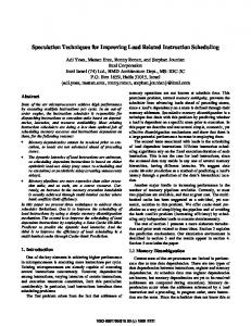
pred completer portion of the mnemonic indicates which value prediction hardware scheme should be used to generate a prediction. Gabbay and Mendelson [5] first introduced specifying opcode directives ("stride" and the "last-value") to highly predictable instructions to reduce the value prediction hardware cost and provide better prediction accuracy. However, since our method has explicit predicting and updating instructions, the predictor type is specified only on the PREDICT and UPDATE instructions, rather than on the predicted instruction itself. The current legal values for pred are: "zero", "last-value", "stride", "stride-2delta", "SAg-last4value". l UPDATE.pred Ry, linktag The UPDATE instruction updates the value predictor with the value in Ry. The linktag is used to allow the hardware to link corresponding PREDICT and UPDATE instructions. UPDATE uses linktag to get the index generated by its corresponding PREDICT to update the value prediction hardware. The pred completer indicates which value predictor is to be updated. One possible implementation of the PREDICT/UPDATE instructions is illustrated in Figure 1 using a stride two-delta value predictor as an example. When the PREDICT instruction generates an index to the value prediction table by hashing the linktag and branch history, this index is stored into the index table at the entry corresponding to the linktag of the PREDICT instruction. The corresponding UPDATE will use the same linktag to lookup the index, which is then used to access the value prediction table. This scheme enables the decoupling of the operations of predicting and updating, so the compiler can schedule the dependent instructions as early as possible. In this approach, the index table only needs to store the indices of the current outstanding PREDICT instructions, so its size can be small. The index table can be direct-mapped or set-associative. The compiler assigns different linktags to each PREDICT and UPDATE pair to help avoid the conflicts in the index table (although, it is not always possible when using dynamic event history as part of the input to the predictor). This new value prediction ISA allows the compiler to incorporate dynamic event history as part of the prediction while retaining the simplicity of a statically scheduled implementation. For the PREDICT instruction, the compiler can alter the number of branch history bits to be hashed on a per-instruction basis to get the best result from global correlation based on profile data. In [13], Nakra et al. presented the hashing of branch history with instruction address (PC) to index the last value table and the stride table. In their experiments, two bits of branch history concatenated with PC provided the best results. In [17], Bekerman et al. suggested that for the load-address predictor, the correlation of the branch history from recent callers is better than xor-ing the PC with the current global history. Unlike the LDPRED instruction, the PREDICT instruction does not speculatively update the value prediction hardware. Therefore, the UPDATE instruction must be executed whether the prediction is correct or not. In the case of the last value predictor, an

4

UPDATE instruction is only necessary in the recovery path since when the prediction is correct, the predictor already has the correct last value in the value table and does not need to be updated. In an implementation of PREDICT/UPDATE, the hardware could choose to implement the different predictor completers as separate hardware structures, or as a combined structure. Examination of the potential implementation alternatives is beyond the scope of this paper. INDEX TABLE

VALUE TABLE

index

linktag

last_value

stride

stride2

index

UPDATE

hash (r1:n,branch_history:b)

Prediction Hardware PREDICT Figure 1. Hardware support for the PREDICT and UPDATE instructions using the stride two-delta predictor as an example.

4.

Revised Value Speculation Scheduling Algorithm

The compiler used for these experiments is based on an experimental IA-64 compiler, with support added for the value prediction ISA and value speculation scheduling (VSS). In this study, value speculation scheduling is performed after pre-pass scheduling and before post-pass scheduling [11]. During pre-pass scheduling the compiler performs global code motion to exploit ILP via control speculation and data speculation. VSS uses the pre-pass schedule to find better split points to break flow dependencies. The value speculation scheduling algorithm utilizes the new PREDICT and UPDATE instructions and selects which instructions are beneficial to value-predict as follows: 1. Perform value profiling to measure the prediction accuracy of instructions using different value prediction algorithms. 2. Compute data dependence graphs and identify critical paths. 3. Apply heuristics to select useful instructions to value-predict. 5

4. Break flow dependencies of the selected instructions and generate recovery code using tail duplication. 5. Perform instruction scheduling. In the following subsections, the details of each step are described. Section 4.1 describes the method of value profiling and the profiled value predictors. Section 4.2 states how to find critical paths in data dependence graphs. Section 4.3 lists the heuristics to select split points. Section 4.4 describes recovery code generation using tail duplication (which allows for efficient generation of recovery code for multiple predictions on a given dependence chain). 4.1. Value Profiling Method and Value Predictors Because the PREDICT and UPDATE instructions use a completer to indicate which value prediction approach should be used, the compiler needs to profile multiple value predictors for all register-writing instructions that it may want to predict. The predictors chosen in this paper, from the simplest to the most complicated, are the zero [15], [20], last value [1], [2], stride [3], [5], [6], [7], stride two-delta [3], [7], and SAg last-four [16] value predictors. The zero predictor is the simplest software value predictor and always predicts the result to be zero. It does not need to use PREDICT and UPDATE instructions, since it only needs to move a zero to the target register. The last value predictor predicts the result to be the last value updated in the prediction table. The stride value predictor adds the difference between to the last two values to the last value as the prediction. The stride two-delta value predictor updates the stride only when the same stride appears twice in a row. The SAg last four-value predictor [16] records the last four results of instructions, and uses confident counters to select which value is used as the prediction. To reduce overhead, the profiler performs multiple predictions and verifications for each predicted instruction in parallel. Therefore, only one profile run is necessary to collect the prediction accuracy of many different value predictors. 4.2. Data Dependence Graph and Critical Path If the split points selected by the value speculation scheduler are not on the critical paths, VSS may increase schedule length by adding one or more extra cycles due to prediction verification and branch overhead. Therefore, the ability to identify instructions on critical paths is important for value speculation scheduling to be effective. Critical path information is obtained from building a data dependence graph (DDG) [10], [11], [12]. After constructing the DDG, a bottom-up depth-first-search (DFS) height assignment and top-down DFS depth assignment algorithm is performed on the DDG. The height of an instruction in the DDG represents the latest schedule cycle required not to delay the execution of other instructions. The depth of an instruction in the DDG is the earliest cycle when the result of this instruction is ready.

6

In this paper, two types of critical paths are used, local critical paths and global critical paths. Local critical paths are critical paths inside each basic block. Global critical paths are critical paths of the entire function. Global critical paths used in this study do not consider the backedges of loops and weights of basic blocks, so the global critical paths only represent the longest path from the entry instruction to the exit instruction, based on the acyclic dependence graph of the function. Most of the instructions on global critical paths are also on local critical paths. Because local critical paths do not consider the dependencies coming from outside of the basic blocks, the calculation of depths and heights inside the basic blocks is different from the calculation of depths and heights at the function level. Instructions that are not on local critical paths are called non local-critical instructions. Instructions with the maximum height are considered as top instructions. Instructions with half of the maximum height are labeled as middle instructions. Section 5.3 presents the predictability of instructions based on their classifications: non-local critical, local critical, and global critical instructions, top and middle instructions, and one-cycle and long-latency instructions. 4.3. Split Point Selection To select better split points for value speculation scheduling, several heuristics are applied. 1. Execution frequency of instructions must be greater than a threshold. 2. The estimated cycle savings by breaking instruction dependencies must be greater than a threshold. 3. Instructions are on critical paths. 4. Instructions are at specific locations within a DDG. 5. Prediction accuracy of instructions must be greater than a threshold. The first heuristic filters out infrequently executed instructions. The second heuristic filters out instruction sequences for which VSS will not reduce critical path length. An example of this is an instruction whose result is fed into a compare instruction which is followed by a branch. Value-predicting this type of sequence cannot reduce execution time, because the value speculation scheduler uses an explicit compare instruction and a branch instruction to verify the prediction of each predicted instructions. The third heuristic selects critical instructions, either on local or global critical paths. The fourth heuristic picks specific instructions to value-predict based on their position in the DDG. In section 5.4, top instructions, middle instructions, and long-latency instructions will be tested for value speculation potential. The fifth heuristic chooses instructions whose values are predictable above a given threshold value. Using these heuristics allows VSS to take into account cost trade-offs of potential benefit versus misprediction cost when incorrect predictions are made.

7

4.4. Recovery Code Generation Using Tail Duplication The generation of recovery code utilizes tail duplication to allow multiple predictions on dependence chains without compromising critical path due to recovery checks. Figure 2 shows an example of revised value speculation scheduling using tail duplication during recovery code generation. Figure 3 shows the original schedule and the VSS schedule of the code in Figure 2. The algorithm is as follows: 1. Insert the predicting instruction, a compare instruction, and the verifying branch right after the predicted instruction. For the software value predictor [15], the predicting instruction is a move, or add instruction. For the hardware value predictor, the predicting instruction is the PREDICT instruction. The destination register number of the predicting instruction is the original destination register, Rold, of the predicted instruction. The verifying branch jumps to recovery code when the value prediction is incorrect. 2. Change the destination register number of the predicted instruction to a free register, Rnew. 3. Split the original basic block into two blocks after the verifying branch. 4. Generate recovery code by duplicating the second half of the split basic block. Insert the move instruction from Rnew to Rold into the recovery block. While this transformation generates unnecessary copies, they will be cleaned up after copy propagation [23] and dead code elimination [23]. 5. Insert the corresponding updating instruction in the bottom basic block and the recovery basic block. The updating instruction is a move or UPDATE instruction according to whether software or hardware value predictors are being used. Tail duplication of recovery code efficiently supports multiple predictions in one dependence chain. For example, in Figure 2, instructions 22 and 25 are both predicted and the maximum cycle savings is obtained. However, the verification of predictions must remain in the dataflow order. Once a prediction is found to be incorrect, all dependent instructions need to be re-executed. Because of this, the UPDATE instruction cannot be scheduled before the verifying branch to ensure the updating of correct values. Using tail duplication for recovery code generation also produces regions without side entrances, which are compatible with superblocks [10] and treegions [12]. In Figure 2, blocks 0, 11, and 13 form a superblock and blocks 0, 11, 13, 12, and 14 form a treegion. Moreover, if tail duplication is applied further down in the control flow graph, large regions will be available to the scheduler. The drawback of using tail duplication for recovery code is that it increases code size and instruction cache misses if not applied carefully. After tail duplication, the scheduler might move an instruction from either the correct prediction path or the recovery path to a dominating block. If this moved instruction has a copy in the other block due to tail duplication, then the copy must be deleted [12].

8

a. Original code BLOCK 0 19 add v3 20 sub v5 21 mov v6 22 shl v7 23 add v8 24 sub v10 25 ld4 v11 26 add v12 27 add v13 28 add v14

= v1, v2 = v3, v4 = v3 = v6, v20 = v5, v7 = v7, v9 = [v8] = v10, v11 = v11, v12 = v12, v13

BLOCK 2

b. VSS code: break flow dependences of operations 22 (shl) and 25 (ld4) in BLOCK 0. BLOCK 0 19 add v3 = v1, v2 20 sub v5 = v3, v4 21 mov v6 = v3 22 shl v15 = v6, v20 31 predict v7 = linktag1 32 cmpne V3 = v7, v15 42 br ?V3 bk12

BLOCK 11 43 update v15, linktag1 23 add v8 = v5, v7 24 sub v10 = v7, v9 25 ld4 v16 = [v8] 45 predict v11 = linktag2 46 cmpne V4 = v11, v16 53 br ?V4 bk14

BLOCK 13 54 update v16, linktag2 26 add v12 = v10, v11 27 add v13 = v11, v12 28 add v14 = v12, v13

BLOCK 12 44 update 33 mov v7 34 add v8 35 sub v10 36 ld4 v11 37 add v12 38 add v13 39 add v14 100 br bk2

BLOCK 14 55 update 47 mov v11 48 add v12 49 add v13 50 add v14 101 br bk2

v16, linktag2 = v16 = v10, v11 = v11, v12 = v12, v13

BLOCK 2

Figure 2. Example of VSS.

9

v15, linktag1 = v15 = v5, v7 = v7, v9 = [v8] = v10, v11 = v11, v12 = v12, v13

a. Original schedule BLOCK 0 0 19 add v3 = v1, v2 1 21 mov v6 = v3 22 shl v7 = v6, v20 2 3 4 5 23 add v8 = v5, v7 25 ld4 v11 = [v8] 6 7 8 9 26 add v12 = v10, v11 10 27 add v13 = v11, v12 11 28 add v14 = v12, v13

20 sub v5 = v3, v4

24 sub v10 = v7, v9

b. VSS schedule BLOCK 0 0 19 add v3 = v1, v2 1 24 sub v10 = v7, v9 22 shl v15 = v6, v20 2 25 sld4 v16 = [v8] 3 4 28 add v14 = v12, v13 5 32 cmpne V3 = v7, v15 BLOCK 11 0 46 cmpne V4 = v11, v16

31predict v7 = linktag1 21 mov v6 = v3 23 add v8 = v5, v7 27 add v13 = v11, v12

45 predict v11 = linktag2 20 sub v5 = v3, v4 26 add v12 = v10, v11

33 mov v7 = v15

42 br ?V3 bk12

43 update v15, linktag1

47 mov v11 = v16

BLOCK 13 0 54 update v16, linktag2 BLOCK 2 …… BLOCK 12 0 34 add v8 = v5, v7 1 36 ld4 v11 = [v8] 2 3 4 37 add v12 = v10, v11 5 38 add v13 = v11, v12 6 39 add v14 = v12, v13 BLOCK 14 0 48 add v12 = v10, v11 1 49 add v13 = v11, v12 2 50 add v14 = v12, v13

44 update v15, linktag1

35 sub v10 = v7, v9

100 br bk2

55 update v16, linktag2 101 br bk2

Figure 3. Original and VSS schedule of code in Figure 2.

10

53 br ?V4 bk14

5. Experimental Results This section provides empirical data gathered during the profiling stage of compilation. Although execution in a full pipeline simulator is desirable, our profiling data is sufficient to measure critical path reduction and potential impact of branch misprediction caused by value prediction checks. Section 5.1 describes the experimental setup. Section 5.2 presents the results of selecting the best predictors on a per-instruction basis, including the branch predictability of the verifying branches for value prediction. Section 5.3 measures the value predictability of instructions based on their classifications. Section 5.4 describes several value prediction heuristics, and measures the benefits of different split point selections based on these heuristics. 5.1. Experimental Setup To measure critical path reductions, an experimental IA-64 machine model was developed that maximizes available resources. This model is not intended to measure the merits of any particular processor implementation or to measure the overall performance of such a machine. Rather, it is intended to allow us to measure potential for value speculation in very wide machines. For this study, the model can issue up to twelve instructions in four bundles each cycle. The latencies of integer instructions are one cycle, except for compare (zero cycles), load (three cycles when hit in cache), shift (three cycles), and getf (three cycles). The latencies of floating-point instructions are two cycles (compare) or eight cycles (load, arithmetic, misc). The model has four floating point units, eight memory units, and twelve ALUs, all of which are fully pipelined. An experimental IA-64 research compiler developed at Intel was used to compile the benchmarks (with support added for VSS and the experimental ISA). In the backend, the compiler is able to generate a value profile, feed the profile data back to the scheduler and perform value speculation scheduling. The profiler instruments the original code by embedding emulated value predictors into it. The instrumented code was run on an IA64 functional simulator to obtain the profile data. All experiments used SPECint95 benchmarks with the input files specified in Table 1. In order to investigate the overall predictability of instructions, all integer register-writing instructions were profiled. SPECint95 Inputs compress 100000 q 2131 gcc stmt.i go 50 9 2stone9.in ijpeg vigo.ppm li train.lsp m88ksim dhry.lit perl scrabbl.pl, primes.pl vortex vortex.raw (with few iterations) Table 1. Inputs of used for SPECint95.

11

5.2.

Results of Selecting the Best Predictors on a Per-Instruction Basis Figure 4 shows the prediction accuracy of our implementation of the zero [15], [20], last value [1], [2], stride [3], [5], [6], [7], stride two-delta [3], [7], and SAg last four-value predictors [16]. The stride two-delta value predictor gets the best average prediction accuracy of 53%. The SAg last four-value predictor is second with a prediction accuracy of 50%. The zero predictor has the lowest prediction accuracy of 12%, but when considering its simplicity, its accuracy is substantial. Note that all predictors in our study have 32K entries independent of their complexity. Figure 4 also shows the prediction accuracy of the best predictors on a per-instruction basis. The completer can select the best predictor for each selected instruction by specifying the appropriate value for the pred completer in the PREDICT instruction. When two different value predictors have the same predictability, the simpler value predictor is used. For this study, the priority order of the predi ctors is: zero, last value, stride, stride two-delta, and SAg last four-value. When the best predictor is chosen on a per-instruction basis among the zero, last value, stride, stride two-delta value predictors, the prediction accuracy is 55%. When the SAg last four-value predictor is added to the available selections, the prediction is 8% higher, at 63%. Note that the effect of adding predictors with different algorithms is substantial. As more types of predictors that operate well in specific instances and better general-purpose predictors are developed, this technique of selecting predictor types on a per-instruction basis will yield increasingly higher returns. In the future work, we will add context predictors such as those in [3], since they are fundamentally different from our current set of predictors. Figure 5 provides a breakdown of how many instructions have a given prediction accuracy using the best value predictors for each instruction. Most static and dynamic instructions are bimodal with prediction accuracy greater then 90% or less than 10%. Since VSS adds one new branch for every predicted instruction, it is important to understand their behavior. If such branches are well-predicted, then recovery cost of value misprediction is small. If they are not well-predicted, recovery is expensive. To measure the predictability of the verifying branches for value prediction in VSS, the profiler models a very simple two-bit saturating counter predictor. If the value prediction is incorrect, the verifying branch will be taken to the recovery code; if the value prediction is incorrect, the branch will fall through. The two-bit saturating counters increment by one, saturating at three when the branch predictions are correct, and decrement by one, saturating at zero when the branches mispredict. The verifying branch is predicted as taken when the saturating counter value is two or three; it is predicted as not-taken when the counter value is zero or one. Figure 6 shows the branch predictability of verifying branches sorted by the value prediction accuracy of instructions. Both highly and poorly value-predictable instructions have very good branch predictability. Instructions with medium value predictability (around 50%) have the lowest branch predictability about or above 50%. Therefore, the branch misprediction penalty only

12

affects medium value predictable instructions. If the value speculation scheduler selects the medium value predictable instructions, it must have larger benefits to compensate the penalty caused by the misprediction of verifying branches. Also note that our experiments are based only on the simple two-bit saturating counter branch predictor. More sophisticated predictors would likely provide significant reduction in branch misprediction thus further decreasing the cost of recovery due to branch misprediciton. Figure 7 shows how often (static and dynamic counts) each of the predictors studied is the best predictor for an instruction. The last value predictor accounts for the largest number of static instructions at about 35%. The zero predictor is the second at about 30% of total static instructions. The remaining static instructions use the SAg last fourvalue, stride two-delta, and stride predictors (in that order). However, if one considers dynamic instruction counts, the SAg last four-value predictor is selected for the most dynamic instructions at about 40%. The second most common is the last value predictor at about 24%, followed by the stride two-delta, zero, and stride value predictors. The stride predictor (non-two delta version) is rarely chosen relative to the last value and stride two delta predictors. Considering the tradeoff of the performance and complexity of value predictors, complex predictors should have a certain amount of performance gain over the simpler value predictor to be selected. Figure 8 shows the same data as in Figure 7, but low priority predictors must win over high priority predictors by at least a 5% margin in prediction accuracy in order to be selected. Using this criterion, the last value predictor accounts for the highest percentage of static and dynamic instructions, 38% and 29%. The SAg last four-value predictor accounts for the second highest dynamic instructions, at 28% (but only 16% of static instructions), which is close to the last value predictor. This type of analysis allows one to factor in relative cost and benefits of using smaller more complex predictors versus larger and simpler predictors. 5.3.

Predictability of Instructions by Classification: Critical vs. NonCritical, Top vs. Middle, One-Cycle vs. Long-Latency The predictability of instructions on the critical path is shown in Figure 9. The definitions of non-local critical, local critical and global critical instructions are given in section 4.2. Figure 9 shows that non-local critical instructions have a higher prediction accuracy than local critical instructions on all benchmarks except m88ksim and perl. The average percentages of static and dynamic non-local critical and local critical instructions are close at about 50%. Global critical instructions have the least predictability, but also account for a smaller percent of overall static and dynamic instructions. Figure 10 shows the predictability of the top and middle instructions on local critical paths. The prediction accuracy of the top instructions is higher than that of the middle instructions. The percentages of the static and dynamic top instructions on local critical paths are much larger than those of the middle instructions on local critical paths. The reason is that the critical paths of DDGs have the shape of inverted trees (wider at the top), so there are many instructions at the top locations of DDGs.

13

Figure 11 shows the predictability of one-cycle and long-latency instructions on local critical paths. The average prediction accuracy of one-cycle instructions is higher than that of long-latency instructions by small amounts for all benchmarks except li and vortex. As expected, one-cycle instructions account for larger static and dynamic distributions than long-latency instructions do, since ALU instructions are more common than loads, shifts, and floating-point instructions. 5.4. Opportunity and Benefit of Split Point Selection Figure 12 shows the static and dynamic percentage of instruction candidates remaining after applying different heuristic filters. After selecting instructions with execution frequency greater than 1000, 30% of static instructions and 83% of dynamic instructions remain. After eliminating instructions whose cycle savings are estimated to be less than two cycles, 20% of static and 50% of dynamic instructions are left. Applying local critical path heuristic, 7% of static and 20% of dynamic instructions are left. Choosing instructions that are at the top, in the middle or long latency leaves 4% of static and 13% of dynamic instructions. Among them, only 2.2% of static and 5.3% of dynamic instructions have a prediction accuracy greater than 50% for some predictors. Figure 13 shows the normalized execution cycles without recovery code in SPECint95. For these results, the value speculation scheduler only inserts the PREDICT and UPDATE instructions into the code. This approach allows us to break flow dependencies to produce an upper bound of critical path reduction without generating recovery checks or branches. The numbers are statically measured by counting cycles and frequencies of basic blocks based on the compiler’s schedule. The prediction accuracy threshold for which we would include an instruction was varied in the experiments. Since we are considering critical path without recovery code, the cost of misprediction is not factored in. Thus, the more instructions selected for VSS, the better the speedup. In a more accurate measurement, the cost of executing the recovery would also need to be considered to get an exact speedup. For these results, we selected instructions with prediction accuracy above 50% as a limit study to provide a basic indicator of potential improvement for VSS. Results in Figure 13 show that predicting long-latency instructions provides the largest reduction in execution cycles for all benchmarks except compress and go. The reason is that the minimum cycle savings of predicting instructions roughly equals the latency of instructions. Predicting the top instructions on local critical paths provides better path reduction than predicting the middle instructions. There are two reasons for this. First, from section 5.3, the top instructions have better prediction accuracy than the middle instructions. Second, predicting the top instructions inside basic blocks can save up to the cost of the entire basic block (if the top instructions are predictable, the compiler will be able to overlap their execution with instructions from previous basic blocks by applying control and data speculation). On the other hand, predicting the middle instructions will generally save at most half of the height of a basic block. The intuition of predicting the instructions in the middle of long global critical paths to reduce the

14

execution time requires careful schedule design. This is because the scheduler must be capable of moving instructions across several branches, and more sophisticated recovery code is required to re-execute all affected instructions. Deeper tail duplication for the recovery code may help reduce these problems. This optimization is left for future work. Figure 14 shows the normalized execution cycles of predicting long latency instructions with recovery code but assuming a prediction accuracy of 100%. The goal of this experiment is to investigate the effects of the verifying branches and the recovery code on the scheduler. Using a prediction accuracy of 100%, the cost of executing the recovery code itself is zero since it is never executed. Thus, if the scheduler is able to get the same estimated cycles through code with recovery and without recovery, then this shows that recovery code does not affect the correctly predicted path. Comparing the long latency results in Figure 13 and the 100% accuracy result in Figure 14, the difference between code with recovery and without recovery ranges from 0.5% to 2.4%. Thus, the verifying branch and recovery code are affecting the code schedule by a small amount. Future work needs to differentiate the recovery code from the normal scheduling region to further reduce the impact. Figure 14 also shows the normalized execution time with recovery code using profiled prediction accuracy. The performance difference between the 100% accuracy and the profiled accuracy comes from the execution of the recovery code. All benchmarks have very small differences, except gcc and ijpeg. If the prediction accuracy increases, the execution frequency of recovery code will be less, and the reduction of cycles will approach the ideal model. This suggests that as more sophisticated value predictors are developed, there is considerable potential for improving critical paths using our scheduling techniques and ISA extensions.

6. Conclusions Value speculation has the potential of increasing instruction level parallelism by breaking true data dependencies. This paper presents a method for integrating value speculation into EPIC ISAs such as IA-64. Although our results indicate value speculation has good potential benefits, our experiment also demonstrates that reaping the benefit will require careful attention to scheduling, profiling, and predictor development. This paper presents a generalized value prediction ISA that improves on the work from [14] by providing for incorporation of dynamic events (such as branch history) and the static selection of predictors for each instruction. The results demonstrate increased predictability by allowing the compiler to select predictors on a per-instruction basis. By using a new recovery code generation technique based on tail duplication, it is possible to generate sequences with multiple recovery checks without severely impacting critical path length (more tuning is still needed). This work also shows that instructions have different predictability based on latency, position within a DDG, and criticality of the instruction. Specific results show that predicting long latency instructions generally provides greater performance enhancements than selecting instructions based upon their position within the DDG.

15

Our results indicate that better predictors are needed to predict the most critical instructions in a program. However, due to the diminishing return of more sophisticated predictors and the compiler’s ability to target only those instructions that get the most benefit from using complex predictors, such complex predictors may not need to be large in order to provide substantial performance enhancements. From our experiments, VSS requires profile data in order to be effective. Work needs to be done to either make such profiles reasonable to collect (following the analogy to [24]) or to develop static estimates to supplant or augment the value profile information (following the analogy to [25]).

7. References [1] M. H. Lipasti, C. B. Wilkerson, J. P. Shen, “Value Locality and Load Value Prediction,” Proceedings of the 7th International Conference on Architecture Support for Programming Languages and Operating Systems, pp. 138-147, October 1996. [2] M. H. Lipasti and J. P. Shen, “Exceeding the Dataflow Limit via Value Prediction,” Proceedings of the 29th International Symposium on Microarchitecture (MICRO-29), pp. 226-237, December 1996. [3] Y. Sazeides and J. E. Smith, “The Predictability of Data Values,” Proceedings of the 30th International Symposium on Microarchitecture (MICRO-30), pp. 248-258, December 1997. [4] B. Calder, P. Feller, and A. Eustace, “Value Profiling,” Proceedings of the 30th International Symposium on Microarchitecture (MICRO-30), pp. 259-269, December 1997. [5] F. Gabbay and A. Mendelson, “Can Program Profiling Support Value Prediction?,” Proceedings of the 30th International Symposium on Microarchitecture (MICRO-30), pp. 270-280, December 1997. [6] K. Wang and M. Franklin, “Highly Accurate Data Value Prediction using Hybrid Predictors,” Proceedings of the 30th International Symposium on Microarchitecture (MICRO-30), pp. 281-290, December 1997. [7] F. Gabbay, “Speculative Execution based on Value Prediction,” EE Department TR #1080, Technion, November 1996. [8] F. Gabbay and A. Mendelson, “The Effect of Instruction Fetch Bandwidth on Value Prediction,” Proceedings of the 25th International Symposium on Computer Architecture, May 1998. [9] D. M. Gallagher, W. Y. Chen, S. A. Mahlke, J. C. Gyllenhall, W. W. Hwu, “Dynamic Memory Disambiguation Using the Memory Conflict Buffer,” Proceedings of the 6th International Conference on Architecture Support for Programming Languages and Operating Systems, pp. 183195, October 1994. [10] W. W. Hwu, S. A. Mahlke, W. Y. Chen, P. P. Chang, N. J. Warter, R. A. Bringmann, R. G. Ouellette, R. E. Hank, T. Kiyohara, G. E. Haab, J. G. Holm, and D. M. Lavery, “The Superblock: An Effective Technique for VLIW and Superscalar Compilation,“ The Journal of Supercomputing, vol. 7, pp. 229248, January 1993. [11] P. P. Chang, D. M. Lavery, S. A. Mahlke, W. Y. Chen, and W. W. Hwu, “The Importance of Prepass Code Scheduling for Superscalar and Superpipelined Proessors,“ IEEE Transactions on Computers, vol. 44, No. 3, pp. 353-370, March 1995. [12] W. A. Havanki, S. Banerjia, and T. M. Conte, “Treegion Scheduling for Wide-Issue Processors,” Proceedings of the 4th International Symposium on High-Performance Computer Architecture (HPCA-4), February 1998. [13] T. Nakra, R, Gupta, and M. L. Soffa, “Global Context-Based Value Prediction,” Proceedings of the 5th International Symposium on High-Performance Computer Architecture (HPCA-5), January 1998. [14] C. Fu, M. D. Jennings, S. Y. Larin, and T. M. Conte, “Value Speculation Scheduling for High Performance Processors,” Proceedings of the 8th International Conference on Architectural Support for Programming Languages and Operating Systems (ASPLOS-VIII), Oct. 4-7, 1998.

16

[15] C. Fu, M. D. Jennings, S. Y. Larin, and T. M. Conte, “Software-Only Value Speculation Scheduling,” Technical Report, Department of Electrical and Computer Engineering, North Carolina State University, June 1998. [16] M. Burtscher and B. G. Zorn, “Exploring Last n Value Prediction,” Technical Report CU-CS-885-99, University of Colorado at Boulder, April 1999. [17] M. Bekerman, S. Jourdan, R. Ronen, and G. Kirshenboim, “Correlated Load-Address Predictors,” Proceedings of the 26th International Symposium on Computer Architecture, May 1999. [18] B. Calder, G. Reinman, and D. Tullsen, “Selective Value Prediction,” Proceedings of the 26th International Symposium on Computer Architecture, May 1999. [19] T. Nakra, R. Gupta, and M. Soffa, “Value Prediction in VLIW Machine,” Proceedings of the 26th International Symposium on Computer Architecture, May 1999. [20] D. Tullsen and J. Seng, “Storageless Value Prediction Using Prior Register Values,” Proceedings of the 26th International Symposium on Computer Architecture, May 1999. [21] S. A. Mahlke, W. Y. Chen, R. A. Bringmann, R. E. Hank, W. W. Hwu, B. R. Rau, and M. S. Schlansker, “Sentinel Scheduling: A Model for Compiler-Controlled Speculative Execution,” ACM Transactions on Computer Systems, vol. 11, no. 4, pp. 376-408, November 1993. [22] Intel Corporation, “IA-64 Application Developer’s Architecture Guide,” (Available from http://developer.intel.com/design/ia64/downloads/adag.htm), May 1999. [23] A. V. Aho, R. Sethi, and J. D. Ullman, Compilers: Principles, Techniques, and Tools. Reading, MA: Addison-Wesley Publishing Company, 1986. [24] K. N. P. Menezes, “Hardware-Based Profiling for Program Optimization,” Ph.D. thesis, Department of Electrical and Computer Engineering, North Carolina State University, 1997. [25] T. Ball and J. R. Larus, “Branch Prediction for Free,” Proceedings of the ACM SIGPLAN ‘93 Conference on Programming Language Design and Implementation, pp. 300-313, June 1993.

17

P r e d ic t io n A c c u r a c y o f D if f e r e n t P r e d ic t o r s z e ro

lv

st

s t2

s a g _ l4 v

b e s t o f ( z e r o , lv , s t , s t 2 )

b e s t o f a ll

Prediction Accuracy

100% 90% 80% 70% 60% 50% 40% 30% 20% 10% 0% c o m p re s s

gcc

go

i jp e g

li

m 8 8 k s im

p e rl

v o rte x

a r it h m e t ic m ean

S P E C in t9 5

Figure 4. Prediction accuracy of different value predictors and the best predictors by selecting among (zero, last value, stride, stride two-delta) and selecting among all (zero, last value, stride, stride two-delta, SAg last four-value) on per-instruction basis. D is tr ib u tio n o f S ta tic In s tr u c t io n s b y P r e d ic tio n A c c u r a c y (U s in g t h e B e s t V a lu e P r e d ic t o r f o r E a c h In s tr u c t io n )

c o m p re s s

gcc

go

ij p e g

li

m 8 8 k s im

p e rl

v o r te x

50%

Instructions

Percentage of Static

60%

40% 30% 20% 10% 0% 100% 90%

90% 80%

80% 70%

70% 60%

60% 50%

50% 40%

40% 30%

30% 20%

20% 10%

10% 0%

P r e d ic tio n A c c u r a c y

D istribu tion of Dynam ic Instructio ns b y Prediction Accuracy (U sin g the Best V alu e P red ictor for E ach Instruction )

Percentage of Dynamic Instructions

com press

gcc

go

ijpeg

li

m 88ksim

perl

vortex

80% 70% 60% 50% 40% 30% 20% 10% 0% 100% 90%

90% 80%

80% 70%

70% 60%

60% 50%

50% 40%

40% 30%

30% 20%

20% 10%

10% 0%

P rediction Accuracy

Figure 5. Percentage of static and dynamic instructions using the best value predictors

18

B r a n c h P r e d ic ta b ility o f V e r ify in g B r a n c h e s

Predictability

c o m p re s s

gcc

go

ijp e g

li

m 8 8 k s im

p e rl

v o rte x

100 90 80 70 60 50 40 30 20 10 0 100% 90%

90% 80%

80% 70%

70% 60%

60% 50%

50% 40%

40% 30%

30% 20%

20% 10%

10% 0%

V a lu e P r e d ic tio n A c c u r a c y

Figure 6. Branch predictability of verifying branches

P e rc e n ta g e o f S ta tic Ins truc tion s S ele c te d b y D iffe re nt P re d ic to rs ze ro

lv

st

st2

sa g_ l4 v

Percentage of Static Instructions

60% 50% 40% 30% 20% 10% 0% co m p re ss

g cc

go

ijp e g

li

m 8 8 ksim

p e rl

vo rte x

a rith m e tic m ean

S P E C int9 5

Percentage of Dynamic Instructions Selected by Different Predictors zero

lv

st

st2

sag_l4v

Percentage of Dynamic Instructions

70% 60% 50% 40% 30% 20% 10% 0% compress

gcc

go

ijpeg

li

m88ksim

perl

vortex

arithmetic mean

SPECint95

Figure 7. Percentage of static and dynamic instructions selected by different value predictors. (Priority is given from zero to SAg last four-value predictors when prediction accuracy is the same.)

19

P ercen tag e o f S tatic In stru ctio n s S elected b y D ifferen t P red icto r (W in by 5% ) zero

lv

st

st2

sag_ l4v

Percentage of Static Instructions

6 0% 5 0% 4 0% 3 0% 2 0% 1 0% 0% c om pres s

g cc

go

ijpe g

li

m 88 ks im

p erl

vo rte x

arithm e tic m ea n

S P E C int9 5

P e r c e n ta g e o f D y n a m ic In s tr u c tio n s S e le c te d b y D iffe r e n t P r e d ic to r s (W in b y 5 % ) z e ro

lv

st

s t2

s a g _ l4 v

Percentage of Dynamic Instructions

60% 50% 40% 30% 20% 10% 0% c o m p re s s

gcc

go

ijp e g

li

m 8 8 k s im

p e rl

v o rte x

a r ith m e tic m ean

S P E C in t9 5

Figure 8. Percentage of static instructions selected by different value predictors. (Priority is given from zero to SAg last four-value predictors. Low priority predictors must win over high priority predictors by 5% of prediction accuracy.)

20

Prediction Accuracy of Critical Instructions non-local critical

local critical

global critical

Prediction Accuracy

100% 80% 60% 40% 20% 0% compress

gcc

go

ijpeg

li

m88ksim

perl

vortex

arithmetic mean

vortex

arith mean

vortex

arithmetic mean

SPECint95

Percentage of Static Critical Instructions non-local critical

local critical

global critical

70%

Percentage

60% 50% 40% 30% 20% 10% 0% compress

gcc

go

ijpeg

li

m88ksim

perl

SPECint95

Percentage of Dynamic Critical Instructions

Percentage

non-local critical

local critical

global critical

70% 60% 50% 40% 30% 20% 10% 0% compress

gcc

go

ijpeg

li

m88ksim

perl

SPECint95

Figure 9. Predictability, static and dynamic percentage of critical instructions (over all integer register-writing instructions).

21

Prediction Accuracy of Top and Middle Instructoins on Local Critical Paths

Prediction Accuracy

Top

Middle

100% 80% 60% 40% 20% 0% compress

gcc

go

ijpeg

li

m88ksim

perl

vortex

arithmetic mean

SPECint95

Percentage of Static Top and Middle Instructions on Local Critical Paths

Percentage

top

middle

40% 35% 30% 25% 20% 15% 10% 5% 0% compress

gcc

go

ijpeg

li

m88ksim

perl

vortex

arithmetic mean

SPECint95

Percentage of Dynamic Top and Middle Instructions on Local Critical Paths top

middle

Percentage

50% 40% 30% 20% 10% 0% compress

gcc

go

ijpeg

li

m88ksim

perl

vortex

arithmetic mean

SPECint95

Figure 10. Predictability, static and dynamic percentage of top and middle instructions on local critical paths (over all integer register-writing instructions).

22

Prediction Accuracy of One-Cycle and Long-Latency Instructions on Local Critical Paths

Prediction Accuracy

1 cycle

long latency

100% 80% 60% 40% 20% 0% compress

gcc

go

ijpeg

li

m88ksim

perl

vortex

arithmetic mean

SPECint95

Percentage of Static One-Cycle and Long-Latency Instructions on Local Critical Paths 1 cycle

long latency

Percentage

50% 40% 30% 20% 10% 0% compress

gcc

go

ijpeg

li

m88ksim

perl

vortex

arithmetic mean

SPECint95

Percentage of Dynamic One-Cycle and Long-Latency Instructions on Local Critical Paths 1 cycle

long latency

60% Percentage

50% 40% 30% 20% 10% 0% compress

gcc

go

ijpeg

li

m88ksim

perl

vortex

arithmetic mean

SPECint95

Figure 11. Predictability, static and dynamic percentage of one-cycle and long-latency instructions on local critical paths (over all integer register-writing instructions).

23

Percentage of Static Instructions Selected by Heuristics freq>1000 freq>1000 && saving>1 freq>1000 && saving>1 && local_critical freq>1000 && saving>1 && local_critical && (top || middle || long) freq>1000 && saving>1 && local_critical && (top || middle || long) && acc>50%

Percentage

60% 50% 40% 30% 20% 10% 0% compress

gcc

go

ijpeg

li

m88ksim

perl

vortex

arithmetic mean

SPECint95

Percentage of Dynamic Instructions Selected by Heuristcs freq>1000 freq>1000 && saving>1 freq>1000 && saving>1 && local_critical freq>1000 && saving>1 && local_critical && (top || middle || long) freq>1000 && saving>1 && local_critical && (top || middle || long) && acc>50%

Percentage

100% 80% 60% 40% 20% 0% compress

gcc

go

ijpeg

li

m88ksim

perl

vortex

arithmetic mean

SPECint95

Figure 12. Percentage of static and dynamic instructions selected by heuristics.

24

Without Recovery Code Model

Normalized Execution Cycles

top

middle

long latency

1.00 0.98 0.96 0.94 0.92 0.90 0.88 0.86 0.84 0.82 0.80 com pres s

gcc

go

ijpeg

li

m 88ksim

perl

vortex

harm onic m ean

SPECint95

Figure 13. Normalized execution cycles without recovery code model. With Recovery Code Model (for Long-Latency Instructions)

Normalized Execution Cycles

100% accuracy

profiled accuracy

1.02 1.00 0.98 0.96 0.94 0.92 0.90 0.88 0.86 0.84 0.82 0.80 compress

gcc

go

ijpeg

li

m88ksim

perl

vortex

SPECint95

Figure 14. Normalized execution cycles with recovery code model.

25

harmonic mean