Eli P. Fenichel, Frank Lupi, John P. Hoehn, and Michael D. Kaplowitz. ABSTRACT. .... Caudill and Groothuis 2005; Carson et al. 1998). However, there is not yet ...
Split-Sample Tests of ‘‘No Opinion’’ Responses in an Attribute-Based Choice Model Eli P. Fenichel, Frank Lupi, John P. Hoehn, and Michael D. Kaplowitz ABSTRACT. Researchers using questionnaires to elicit preferences must decide whether to include response options that allow respondents to express ‘‘no opinion.’’ Using a split-sample design, we explore the implications of alternative answer formats including and not including no-opinion responses in an attribute-based choice experiment. The results indicate that using multiple no-opinion responses may enable researchers to differentiate between respondents who choose no-opinion options due to satisficing and those expressing utility indifference. Existing literature suggesting no-opinion responses may be treated as ‘‘no,’’ but our results show treating no-opinion responses as no yields substantially disparate preference estimates. (JEL C25, Q24, Q25, Q51)
I. INTRODUCTION
In surveys eliciting stated preferences, some respondents opt to answer a choice question with a response such as ‘‘don’t know,’’ ‘‘not sure,’’ or ‘‘would not vote.’’ These responses are variants of the ‘‘no opinion’’ responses discussed in the broader survey research literature (Krosnick 2002). Treatment of no-opinion responses in stated preference studies has largely focused on studies that use the contingent valuation method (CVM). The attribute-based method (ABM), also called choice experiments or stated choice, is a comparatively new technique that is related to CVM (Louviere, Hensher, and Swait 2000; Foster and Mourato 2003; Holmes and Adamowicz 2003). The ABM presents respondents with a set of attributes of a good, where typically one attribute is price. The attributes and prices are varied across respondents. This differs from CVM, where typically only Land Economics N May 2009 N 85 (2): 349–363 ISSN 0023-7639; E-ISSN 1543-8325 E 2009 by the Board of Regents of the University of Wisconsin System
Land Economics leco-85-02-09.3d 5/1/09 17:36:13
price is varied across respondents. ABM, therefore, allows the researcher to value the implicit price for each attribute, much like a hedonic price study (Holmes and Adamowicz 2003). Typically, CVM and ABM use discrete choice responses, and as a result random utility models can be used in the estimation of both methods. Indeed, CVM may be considered a special case of ABM (Boxall et al. 1996). Although some research has addressed treatment of noopinion responses in CVM studies, this paper represents a first effort to understand the significance of no-opinion responses in ABM. In many ABM-based studies, respondents are asked to choose between two or more attribute-price sets. This is similar to the referendum-style questions commonly used in CVM, especially in the case where one attribute-price set is treated as a status quo. The National Oceanic and Atmospheric Administration (NOAA) panel recommended including a ‘‘no vote’’ option for binary choice CVM studies (Arrow et al. 1993). While, this recommendation has spawned a growing body of research on how to treat ‘‘would not vote’’ and other types of no-opinion responses in the CVM literature, the issue has received less attention in ABM studies. The increasing use of The authors are, respectively, research associate, Quantitative Fisheries Center, Department of Fisheries and Wildlife; associate professor of Agricultural, Food, and Resource Economics and Fisheries and Wildlife; professor of Agricultural, Food, and Resource Economics; and associate professor of Community, Agriculture, Recreation, and Resource Studies. All are at Michigan State University. The research reported here was supported in part by the Science to Achieve Results (STAR) Program, U.S. Environmental Protection Agency, and the Quantitative Fisheries Center at Michigan State University. This is contribution number 2009-01 of the Quantitative Fisheries Center. The authors are solely responsible for any errors.
349
350
Land Economics
ABM studies for policy decisions and valuation (e.g., Birol, Karousakis, and Koundouri 2006) motivates a more careful examination of the use and analysis of noopinion responses in ABM studies. This seems especially relevant since meta-analyses have shown that methodology can affect welfare estimates (Brander, Florax, and Vermatt 2006; Johnston et al. 2006). Therefore, researchers’ design and treatment of no-opinion responses, along with broader methodological design, must be considered if ABM welfare results are to be used for benefit transfer. There is growing evidence in the CVM binary choice literature that no-opinion responses should not be treated as ‘‘for’’ votes (Groothuis and Whitehead 2002; Caudill and Groothuis 2005; Carson et al. 1998). However, there is not yet agreement as to whether no-opinion responses should be treated conservatively as ‘‘against’’ votes (Carson et al. 1998; Krosnick 2002), or whether no-opinion responses may represent cognitive difficulties, potentially resulting from utility indifference, and therefore should be treated as a truly unique response (Krosnick et al. 2002; Evans, Flores, and Boyle 2003; Alberini, Boyle, and Walsh 2003; Caudill and Groothuis 2005; Champ, Alberini, and Correas 2005). Furthermore, those who support treating no-opinion responses in CVM as unique responses seem to largely base their recommendation on improving econometric efficiency, with few researchers arguing that treating such responses as ‘‘against votes’’ (the conservative approach) yields inconsistent estimates. Groothuis and Whitehead (2002) observe that treating no-opinion responses in CVM as unique or ‘‘against’’ votes may depend on whether the study is attempting to measure willingness to pay (WTP) or willingness to accept (WTA). Arguments for treating no-opinion responses as unique responses in estimation are often based on Wang’s (1997) hypotheses on why respondents choose no-opinion responses. Wang (1997) posits that there are four general categories of respondents who choose no-opinion responses: (1) those who
Land Economics leco-85-02-09.3d 5/1/09 17:36:20
May 2009
reject the CVM scenario, (2) those who know their preference and decline to answer, (3) those who make an effort and are truly unsure, and (4) those who do not make an effort and are therefore unsure. Krosnick et al. (2002) also examine why a respondent may choose a no-opinion response. Their evidence suggests that noopinion responses may result from satisficing; that is, the ‘‘work’’ involved with answering the question is so great that the respondent chooses a no-opinion response because it involves the least work or the lowest risk for him or her.1 Krosnick et al. (2002) also discuss an alternative hypothesis for a respondent’s no-opinion response: that a respondent’s optimizing process may result in true indifference. In this case, the respondent is truly unsure when the choices are close in terms of the associated net benefits or welfare yields. Accordingly, a respondent may reply with a no-opinion response because he or she is indifferent in a utility sense. However, it is unlikely that there is a clear line between no-opinion responses resulting from optimizing and from satisficing, since a respondent may begin optimizing but may ‘‘give up’’ before reaching true indifference. Investigations by Alberini, Boyle, and Welsh (2003), Caudill and Groothuis (2005), and Evans, Flores, and Boyle (2003) have been aimed at improving estimation efficiency through sorting noopinion responses into response categories for estimation purposes. This sorting has focused on identifying and making use of responses that seem to fall into Wang’s (1997) latter two unsure categories or that may be cases of optimizing as per Krosnick et al. (2002). However, there has been little effort to sort no-opinion responses that may be the result of other phenomena, such as no-opinion responses that result from respondents being unsure because of utility indifference or satisficing. Moreover, most of the work has been focused on ordinal 1 Work requirements may range from reading the survey and understanding the question to evaluating preferences.
350
85(2)
Fenichel et al.: Split-Sample Tests of ‘‘No Opinion’’ Responses
FIGURE 1 NONTRIVIAL ATTRIBUTE COMPARISONS LIKE THOSE COMMON IN MAIN-EFFECTS DESIGNS: OPEN CIRCLE, BASELINE SCENARIO; SOLID CIRCLES, SAMPLE OF THE POSSIBLE ALTERNATIVES THAT ARE NOT UNIFORMLY BETTER OR WORSE IN THEIR INDIVIDUAL ATTRIBUTES; GRAY AREAS, ATTRIBUTE COMBINATIONS THAT ARE BETTER (WORSE) IN ALL ATTRIBUTES
polychotomous-choice and multibounded questions, which introduce other types of difficulties (Vossler and Poe 2005). The literature on ABM does contain a related, but logically distinct, strain of research. In some ABM studies, respondents are presented with sets of alternatives composed of varied attributes and an answer set that includes a ‘‘none’’ alternative (Louviere, Hensher, and Swait 2000) or an ‘‘opt out’’ alternative (Boxall et al. 1996). In the setting of a product choice, the none option might be treated as a ‘‘don’t buy’’ decision (e.g., Birol, Karousakis, and Koundouri 2006). In a recreational site choice context, the none option might represent a no-trip decision, or it might represent a trip to a site not included in the choice set (Banzhaf, Johnson, and Mathews 2001). In other settings, the none option may be considered a choice to maintain the status quo. Typically, researchers explicitly model this type of alternative as one of the elements in a multinomial choice model (Birol, Karousakis, and Koundouri 2006). In contrast, here we consider a distinct case in the ABM, in which a failure of respondents to choose
Land Economics leco-85-02-09.3d 5/1/09 17:36:21
351
an alternative is not a choice for the status quo. Instead, we examine the setting in which respondents’ failure to choose one of the ABM alternatives is akin to a noopinion response. Some question also remains about the comparability of ABM studies to CVM studies (Stevens et al. 2000; Foster and Mourato 2003). As a result of their explicit substitutes, ABM studies may be cognitively more difficult than CVM studies and may ask respondents to explore their preferences in more detail (Stevens et al. 2000). Alternatively, CVM studies tend to be one dimensional (i.e., apart from any scope tests, all else is held constant for the respondent), while ABM studies involve multidimensional trade-offs that may result in a larger number of respondents who honestly don’t know or are closer to indifference relative to CVM. The proportion of no-opinion responses may be further exacerbated in ABM studies by the common practice of using a main-effects attribute design (e.g., Birol, Karousakis, and Koundouri 2006). Such designs can improve econometric efficiency but may place respondents close to utility indifference for a large share of the alternatives in the design, thereby increasing cognitive difficulty. Figure 1 illustrates the point that when using a main-effects design, few attribute combinations would arise in the gray area that represents alternatives where the levels of each attribute are strictly better (or worse) than those of another design alternative. Choices among alternatives with strictly better (worse) attributes should be cognitively easy. Instead, many ABMs will involve more difficult comparisons of alternatives with more subtle attribute level differences (some better, some worse), making indifference more likely. If the meaning of a no-opinion response is unclear to the researcher, then increased econometric benefits from categorizing or sorting those no-response options will be lost. There have been no studies examining reclassifying no-opinion responses in ABM as ‘‘no’’ responses, which is considered a conservative classification in CVM. That is,
351
352
Land Economics
it remains to be tested whether treating noopinion responses in ABM as ‘‘no’’ responses generates estimates that are consistent with similar surveys where a noopinion option is not offered. Therefore, this paper examines two research questions concerning no-opinion responses in ABM studies. First, does recoding no-opinion responses as ‘‘against’’ (our ‘‘no’’ response choice) provide estimates consistent with those derived from a survey instrument that was the same in every respect expect for an absence of any no-opinion response category? Secondly, does offering respondents two qualitatively different no-opinion responses allow expressions of welfare indifference to be sorted from expressions of no opinion for other reasons? This latter issue may be generalizable to CVM because it attempts to distinguish Wang’s (1997) third type of response (indifferent or too close to call) from Krosnick et al.’s (2002) satisficing or other variants of no opinion. II. SURVEY INFORMATION
A binary choice ABM survey was implemented using a web-based method with a split-sample design. In addition to the usual experimental design of the attributes, there were four unique versions of the ABM survey that differed in the response options (treatments) respondents received for their choice questions: 1. 2. 3. 4.
‘‘Yes’’ and ‘‘no’’ [yes/no treatment] ‘‘Yes,’’ ‘‘no,’’ and ‘‘too close to call’’ (TCC) [TCC treatment] ‘‘Yes,’’ ‘‘no,’’ and ‘‘not sure’’ (NS) [NS treatment] ‘‘Yes,’’ ‘‘no,’’ TCC, and NS [all-options treatment]
For each treatment, the last expression, in square brackets, is what each treatment is called in this paper. Collectively, the NS and TCC responses are referred to as no-opinion responses as a shorthand to refer to respondents who did not explicitly choose yes or no in the choice scenario. The TCC response is hypothesized to reflect choice situations for respondents close to utility indifference.
Land Economics leco-85-02-09.3d 5/1/09 17:36:21
May 2009
The web-based ABM survey elicited preferences for inland, freshwater wetland mitigation from adult Michigan residents. Access to potential respondents was purchased from Survey Sampling International (SSI), which maintains a web-based panel of individuals who have agreed to complete an occasional online questionnaire in return for participation in a prize lottery. The SSI panel is a sample of potential survey respondents with known demographic characteristics. The response treatments were randomly assigned to respondents to prevent systematic differences across treatment response groups.2 Similarly, all four of the response treatments utilized the same experimental design for the survey attributes. E-mail invitations to the SSI panel of potential respondents resulted in 3,454 visits to the welcome page of the web-based questionnaire. Of those potential respondents who visited the survey’s welcome page, 58% completed at least one wetlands mitigation choice question and provided some demographic information. All together, there were 9,753 usable choice question responses for the reported analyses. The questionnaire was developed using a series of focus groups and pretest interviews (described by Kaplowitz, Lupi, and Hoehn 2004) and used a policy setting and set of choice questions that follow the paper instrument discussed by Lupi, Kaplowitz, and Hoehn (2002). Each respondent was presented with the characteristics of a common wetland that had already been approved for drainage (drained wetland) and the characteristics of a wetland being proposed as compensation (restored wetland) for the wetland to be drained. The attributes of the wetlands presented to respondents were wetland type (wooded, marsh, mixed), size (acres), public access attributes, and habitat attributes (these 2 The percentage of respondents living in a selfdescribed rural region ranged from 28% to 30%. Average income ranged between $52,000 and $55,000 annually. Percentage of respondents with a college education ranged from 28% to 32%. Average age ranged from 42.2 to 42.9 years, and percentage male ranged from 40% to 47%.
352
85(2)
Fenichel et al.: Split-Sample Tests of ‘‘No Opinion’’ Responses
353
TABLE 1 RESPONSE DATA Survey Version/ Response Treatment Yes/no TCC NS All options
Proportion of Total Responses 1,586 1,683 1,619 3,000
Yes
No
TCC
NS
0.590 0.537 0.553 0.467
0.410 0.272 0.288 0.287
– 0.191 – 0.164
– – 0.159 0.082
No Opinion – 0.191 0.159 0.246
Note: TCC, too close to call; NS, not sure.
included habitat for songbirds, wading birds, amphibians and reptiles, and wild flowers). The respondents were told: We need your opinion as a member of the citizens’ panel on five restoration cases. The cases represent the kind of decisions that are made every day by wetland restorers. In each case, the project to drain a common type of wetland has already been approved. The only question is whether quality and quantity of a restored wetland is enough to make up for the loss of the drained wetland. If the restored wetland is approved, the restoration project goes forward. If the restored wetland is not approved, the restoration project goes back to the drawing board. A revised project will be reviewed by a different citizens’ panel. In your opinion, is the restored wetland good enough to offset the loss of the drained wetland?
The question was framed this way to address a tendency, found during survey development, for some respondents to vote against a project without weighing the attributes of the alternatives as a way of blocking development and wetlands drainage. Each respondent was asked to make five wetland comparisons, but each respondent had the same response treatment (answer set) for each of his or her choice questions. Further details of the survey design, administration, and general results were presented by Hoehn, Lupi, and Kaplowitz (2004), and a sample instrument is available upon request from the authors.
III. RESPONSE FREQUENCY ANALYSIS
The study design included four different response treatments. Response statistics for the completed choice questions for each treatment are presented in Table 1.3 As expected, the all-options response treatment resulted in the highest proportion of noopinion responses (25%). Chi-square tests were used to compare the proportion of noopinion responses across the three survey response treatments that offered no-opinion responses (Table 2).4 Table 2 shows that the probability of a no-opinion response is significantly different when all four response options are presented to respondents, as compared to instances in which only one type of no-opinion response is available to respondents. This is true at all common significance levels. These results imply that respondents are more likely to choose a no-opinion response when both the TCC and NS options are available. A chi-square test comparing the TCC response treatment and the NS response treatment yielded a low p-value (,0.016). 3 A total of 4,865 responses were received for the alloptions treatment, but 1,865 of these observation were randomly selected and reserved for later use in assessing the model predictions. 4 All chi-square tests use the Yates correction for variables coming from a binomial distribution (Zar 1996).
TABLE 2 CHI-SQUARE TESTS COMPARING PROPORTION OF NO-OPINION RESPONSES NS vs. TCC x2 statistic p-value
All Options vs. NS
5.8360 0.0157
47.1749 0.0000
Note: TCC, too close to call; NS, not sure.
Land Economics leco-85-02-09.3d 5/1/09 17:36:21
353
All Options vs. TCC 18.3050 0.0000
354
Land Economics
May 2009
TABLE 3 RATIO OF YES TO NO RESPONSES BY RESPONSE TREATMENT Ratio of Yes to No Survey Version/ Response Treatment
No Opinion, Dropped
Yes/no TCC NS All options
No Opinion, Pooled with No
1.44 1.97 1.92 1.63
– 1.16 1.24 0.88
Note: TCC, too close to call; NS, not sure.
This result suggests that the TCC and NS response options are not viewed as equivalent response options by respondents, and indicates that the wording of no-opinion options may matter. In addition to the four response treatments, there were two different data coding treatments, one treating no-opinion responses as no, and the other dropping noopinion responses from the data set. As a result, we ended up with seven sets of choice data with different yes/no ratios (Table 3). The ratio of yes to no responses is important because it affects the estimated parameters, especially the constant term, in common methods for implementing random utility models (e.g., logit models). Carson et al. (1998) used chi-square tests to determine the effect of no-opinion responses on the proportion of yes to no responses in a CVM study. We conducted a similar analysis for the ABM data (Table 4 section A). The proportion of yes to no responses was significantly different, at the 95% confidence level, between surveys
treatments that did not allow respondents to express ‘‘no opinion’’ and those that offered either TCC or NS as response options. A chi-square analysis comparing the ratio of yes to no in the yes/no response treatment to the all-options response treatment yielded a difference with a p-value of 0.07. This difference may not be significant at the traditional 95% confidence level but may yield different economic results; in other words, the yes’s and no’s from these two groups may produce different estimates of WTA. No-opinion responses were then pooled with no responses, and the yes/no ratio was retested against the yes/no ratio from the yes/no treatment (Table 4 section B). All chi-square tests for all of these comparisons yielded significant differences (p , 0.05). This result implies that pooling no-opinion responses with no responses, as suggested by Carson et al. (1998), results in significantly different yes/no ratios and contrasts with the findings of Carson et al. (1998) for CVM. It remains unclear in the all-options
TABLE 4 CHI-SQUARE RESULTS FOR COMPARING YES/NO RATIOS Comparison
Yes/No and TCC
Yes/No and NS
Yes/No and All Options
A. The ratio of yes to no responses with no-opinion responses dropped compared to yes/no treatment 16.4712 13.6764 3.2734 x2 statistic p-value 0.0000 0.0002 0.0704 B. The ratio of yes to no responses with no-opinion responses coded as no compared to yes/no treatment x2 statistic p-value
9.3238 0.0023
4.4130 0.0357
62.4845 0.0000
C. The ratio of yes to no responses compared between no-opinion treatments (no-opinion responses dropped) x2 statistic p-value
0.0961 0.7566
6.8678 0.0088
Note: TCC, too close to call; NS, not sure.
Land Economics leco-85-02-09.3d 5/1/09 17:36:21
354
4.9850 0.0256
85(2)
Fenichel et al.: Split-Sample Tests of ‘‘No Opinion’’ Responses
response treatment whether both TCC and NS pulled equally from the yes and the no responses. We also compared yes/no ratios after dropping the no-opinion responses from the data set across the three noopinion survey treatments (Table 4 section C). The ratio of yes to no responses did not change significantly when TCC or NS was offered as the no-opinion response option. The ratio of yes to no responses in the alloptions survey treatment was significantly different at the 95% confidence level compared to the ratio of yes to no responses when only one no-opinion response option was presented (TCC and NS survey treatments). When more than one no-opinion option was presented, the ratio of yes to no responses differed significantly. These results indicate that survey participants are influenced by the phrasing, language, or number of no-opinion response items, supporting the hypothesis that various no-opinion responses may represent unique types of responses. Further, these results suggest that no-opinion responses do not pull evenly from the yes and the no responses and that, unlike Carson et al.’s (1998) CVM study, these responses do not consistently pull from the no responses. It does appear, in this instance, that no-opinion responses pull some from the yes responses and more heavily from the no responses (see Table 1). Moreover, no-opinion responses seem to pull more evenly from the yes and the no responses when both TCC and NS were presented as options as opposed to when only one type of no-opinion response was available (Table 1). It appears that the marginal impact of adding a second noopinion response option is to pull more responses from the yes than the no responses, even though the first no-opinion response option appears to draw more from the no than the yes responses. Three potential scenarios seem to explain the apparent divergence in results between this ABM study and previous CVM studies. First, the underlying ABM study focuses on respondents’ WTA compensation (Gro-
Land Economics leco-85-02-09.3d 5/1/09 17:36:21
355
othuis and Whitehead 2002) as measured by in-kind trade-offs. Second, there may be something unique to the ABM response format that is different from CVM studies. Thirdly, it is possible that the additional noopinion response option causes responses to pull more evenly from both the yes and the no pools. The response ratios obtained imply that TCC and NS responses are good substitutes when only one response option is available to respondents. When both TCC and NS are present, the results appear to support the hypothesis that a TCC response may involve, perhaps, an attempt by respondents to optimize. It is possible that one effect of including no-opinion response options would be to lower item nonresponse rates for the choice question. The item nonresponse rates for the survey treatments were yes/no (0.7%), TCC (1.5%), NS (0.4%), and all options (0.8%). These differences are statistically significant (p , 0.0001). Interestingly, the TCC item nonresponse rate is higher than that of the NS treatment. This result provides some further evidence that the TCC response option is being used by respondents differently than the NS response option. Overall though, none of the treatments had substantial levels of item nonresponse. Response ratios provide some information about no-opinion responses in ABM studies. But the ultimate purpose of ABM studies is to examine welfare estimates and preference orderings. Therefore, in the next section we test whether different question response treatments or data coding treatments result in estimates that imply different compensation measures or different preference ordering. IV. EFFECTS ON WELFARE
The wetlands mitigation survey used in this study asked respondents to make an inkind trade-off between acres of drained and restored wetlands. In essence, respondents were asked if the restored wetland, with specified attributes, would compensate for the loss of an existing wetland, a context
355
356
Land Economics
that mirrors the wetland permitting and mitigation process in the United States. Therefore, wetland acres are the unit of currency for this analysis. The drained and restored wetlands presented to respondents differed in their attributes. The various wetland quality attributes included in the choice sets act to shift demand for wetland acres. Responses were coded into 11 response variables. These variables included change in wetland acreage, dummy variables for capturing changes in wetlands’ general vegetative structure, public access, and habitat conditions for amphibians, songbirds, wading birds, and wildflowers (changes could between poor and good, or good and excellent). Changes in wetland acres were recorded as the change in the total number of acres. Dummy variables were coded as 1 for a positive change, 0 for no change, and 21 for a negative change. Changes from poor to excellent were indicated by both the poor to good and good to excellent dummy variables being coded as 1 (other coding followed this pattern). A change from no access to access was coded as 1 (21 for the other direction), and changes in wetland type were coded as 1 for a change. In-kind welfare measures were estimated using random utility theory (Holmes and Adamowicz 2003). The seven data sets (combinations of each survey and data coding treatment) were fit using a random effects logit model that addressed the panel data. The random effects logit, estimated by maximum likelihood, fits parameter values so that the probability of response i being yes (indicated by 1 and meaning that the restored wetland offset the loss of the drained wetland in comparison i), from respondent j is given by Probðyesi ~ 1Þ ~Lða z bðACRESrestored { ACRESdrained Þ � z cDXi z vj ,
where L is the logistic cumulative distribution function; a and b are scalar estimated parameters; c is an estimated vector of parameters corresponding to changes in
Land Economics leco-85-02-09.3d 5/1/09 17:36:22
May 2009
wetlands attributes, DXi; and vj is a random effect that accounts for the lack of independence among responses provided by the same respondent. All seven models fit the data, with loglikelihood ratio tests against a model with a single choice dummy being significant at all common significance levels. Each model included all variables, though not all estimated coefficients were significantly different from zero at the 95% confidence level. In all models the parameter associated with the change in wetland acres was significantly greater than zero at the 95% confidence level. Parameter ratios were used to calculate in-kind marginal implicit prices in acres of restored wetland (Table 5). For the constant term, the marginal implicit price is the change in acres required to maintain the same level of utility, ceteris paribus. That is, one acre of restored wetland would adequately compensate for one acre of drained wetland if the WTA estimate were zero. In cases where only yes and no options were presented, a restored wetland could have up to just over eight fewer acres for each acre of the drained wetland, ceteris paribus, before respondents would prefer the drained wetland (Table 5, first row). This counterintuitive result for the constant term is likely a consequence of the linear form for the utility function and perhaps a result of the incentive properties of the question. The linear form of the utility function is the most common form in the literature, and hence it is most relevant for our comparison of response options. However, when one alters the underlying responses in a way that increases the share of yes responses, then all else equal, it lowers the implied compensation. It is well known in discrete-choice contingent valuation that the linear form does not ensure estimated welfare measures are positive and can lead to counterintuitive results (Haab and McConnell 2002). Additionally, the question format may have encouraged respondents to accept fewer acres to ensure that some type of restoration project was approved as opposed to not being certain of
356
85(2)
Fenichel et al.: Split-Sample Tests of ‘‘No Opinion’’ Responses
357
TABLE 5 MARGINAL IMPLICIT PRICES OF ATTRIBUTES ASSOCIATED WITH THE WILLINGNESS-TO-ACCEPT (WTA) IN-KIND ACRES COMPENSATION FOR DRAINED WETLANDS TCC
Survey Type Handling of no opinion WTA, ceteris paribus Change of wetland type Access Amphibian p R g Songbird p R g Wading bird p R g Wild-flower p R g Amphibian g R e Songbird g R e Wading bird g R e Wild-flower g R e
Yes/No 28.42 5.86 26.65 27.40 210.70 27.69 23.79a 25.49 25.47 25.49 22.27a
Pooled with No
NS
Discarded
a
22.54 5.79 24.89 23.25a 23.36 27.68 23.16a 24.39 23.41 22.75 24.12
211.96 7.76 25.53 24.02 24.84 27.56 22.44a 23.95 22.19a 23.57 24.52
Pooled with No a
23.55 4.80 27.48 28.78 210.24 29.50 23.66a 26.92 21.89a 24.53 24.26
All Options
Discarded
Pooled with No
211.56 4.45 27.03 29.44 211.02 210.20 23.44a 26.79 22.90 24.98 23.81
4.81 2.75 25.64 27.32 24.97 25.99 22.23a 25.24 25.24 23.37 21.53a
Discarded 25.16 2.66a 27.37 26.74 26.96 26.72 21.55a 25.37 25.30 23.50 21.59a
Note: Values in this table represent the parameter estimate associated with the listed variable divided by the parameter for changes in area, p R g 5 poor to good, and g R e 5 good to excellent. TCC, too close to call; NS, not sure. a Marginal implicit prices that were not significantly different from zero at the 95% confidence level. Confidence intervals were determined by bootstrapping the dataset and reestimating the model 10,000 times for each model.
getting restoration. That is, it is possible that some respondents perceived a no vote as ‘‘dragging out’’ the process and reducing the chances of any mitigation. Examination of response patterns of respondents revealed that those who chose the same response throughout the choice experiment (serial respondents) were mostly likely to choose yes, supporting this hypothesis.5 The WTA estimates, ceteris paribus, varied greatly across response treatments. In treatments with no-opinion responses, dropping the no-opinion responses from the analysis yielded WTA estimates that were closest to those derived from the yes/no format. The WTA estimates showed that substantially less compensation was demanded by respondents 5 Serial respondents answered all five questions using the same response: in the yes/no survey response treatment 15.5% and 9.5% of respondents serially answered yes and no, respectively; in the TTC survey response treatment 11.9%, 2.7%, and 3.3% of respondents serially answered yes, no, and TTC, respectively; in the NS survey response treatment 13.1%, 4.7%, and 4.4% of respondents serially answered yes, no, and NS, respectively; and in the all-options survey response treatment 7.8%, 3.7%, 0.5%, and 2.8% of respondents serially answered yes, no, TCC, and NS, respectively (about 4% of respondents evenly distributed across survey treatments answered fewer than five questions and were not considered to be serial responders).
Land Economics leco-85-02-09.3d 5/1/09 17:36:22
when no-opinion responses were dropped as opposed to pooled with no. Recoding the no-opinion responses as no in the alloptions response treatment makes the ratio of yes to no less than 1 (Table 1) and causes the WTA to be positive, that is, one acre drained required more than one acre restored to offset the loss.6 An important aspect of the ABM is that it allows the relative importance of the attributes to be ranked. Recoding the data changed the yes/no ratio and affected the constants, as expected. However, recoding the data should not affect the ranking of attributes if no-opinion responses represent satisficing. To investigate if recoding affected the relative importance of attributes, the marginal implicit prices associated with each attribute variable (Table 5) were ranked from the largest marginal impact 6 Under maximum likelihood estimation in the logit model, the estimated constant parameter ensures that the average of the predicted probabilities of yes answers matches the sample share of yes answers. To the extent that the no-opinion answers are not being explained by the other parameters of the models, the under the recoding of responses the newly estimated constant adjusts to match the new sample shares. Thus, recoding of no-opinion responses as no responses has the clear effect of lowering the constant and hence lowering the marginal implicit prices.
357
358
Land Economics
May 2009
TABLE 6 RANKING OF THE MARGINAL IMPLICIT PRICES AND THE MAXIMUM DIFFERENCE IN RANKING ACROSS MODELS; RANKINGS OF 1 HAD THE LARGEST MARGINAL EFFECT AND 10 HAD THE LOWEST MARGINAL EFFECT TCC
Survey type Handling of no opinion Change of wetland type Access Amphibian p R g Songbird pR g Wading bird p R g Wild-flower p R g Amphibian g R e Songbird g R e Wading bird g R e Wild-flower g R e
Yes/ No
Pooled with No
NS
Discarded
Pooled with No
All Options
Discarded
Pooled with No
Discarded
Median Rank
Maximum Difference
10
10
10
10
10
10
10
10
0
4 3 1 2 8 6 7 5 9
2 7 6 1 8 3 5 9 4
2 5 3 1 8 6 9 7 4
4 3 1 2 8 5 9 6 7
4 3 1 2 8 5 9 6 7
3 1 6 2 8 4 5 7 9
1 3 2 4 9 5 6 7 8
3 3 2 2 8 5 7 7 7
3 6 5 3 1 3 4 4 5
Note: TCC, too close to call; NS, not sure; p R g 5 poor to good; g R e 5 good to excellent.
to lowest marginal impact (Table 6).7 The maximum difference in rank was used to determine if the different response and data coding treatments maintained consistent preference ordering. Low maximum differences indicate that all models order the preference for a given attribute similarly. Changing wildflower habitat from poor to good had the lowest maximum difference in rank (excluding a change in wetland type, which increased the desired amount of compensation), though these marginal implicit prices were not significantly different from zero at that 95% confidence level. Improving wading bird habitat from poor to good and increasing access consistently ranked highly (median rank of 2 and 3, respectively) and had a low maximum difference (maximum difference of 3 for both). Other attributes that generally ranked highly, however, did so less consistently, largely due to TCC responses. For example, changes in songbird habitat from poor to good also had a high median rank, 2, but had a maximum difference in ranks of 5. This 7 It is expected that marginal implicit price for a positive change in wetland quality would result in a negative implicit price, that is, less acres of restored wetland would be need, if the restored wetland were of higher quality. Inspection of Table 5 reveals that all of the quality attributes had the expected signs, though not all were significant.
Land Economics leco-85-02-09.3d 5/1/09 17:36:22
difference is driven by the ranks associated with the TCC and all-options response treatment when the no-opinion responses are pooled with no, thereby providing evidence that TCC response may not represent satisficing. In contrast, the attribute ranks for the NS format are identical for all attributes, and very similar to the yes/ no format, regardless of whether the NS was pooled with no or dropped. The preference ordering for the all-options treatment when the no-opinion responses are dropped is also similar to the orderings for the yes/no treatment and both NS treatments. Rank correlations between treatments provide further evidence that TCC and NS responses are not used interchangeably (Table 7). Preference ordering was generally correlated across all treatments except the response treatment TCC, with the recoding of TCC responses as no. Moreover, both NS response treatments when compared to the yes/no response treatment had correlation coefficients of 0.94—the highest correlation that yes/no had with any of the response treatments. The finding of the similarity of results for the NS models and the yes/no treatments is similar to the finding of Carson et al. (1998) for CVM. The results also provide some evidence that NS by itself acts more like a no response, due to satisficing, than an expression of indifference.
358
85(2)
Fenichel et al.: Split-Sample Tests of ‘‘No Opinion’’ Responses
359
TABLE 7 RANK CORRELATION RESULTS BETWEEN TREATMENTS
Yes/No Yes/no TCC pooled with no TCC discarded NS pooled with no NS discarded No-opinion pooled with no No-opinion Discarded
TCC Pooled with No
TCC Discarded
NS Pooled with No
NS Discarded
All Options, No-Opinion Pooled with No
All Options, No-Opinion Discarded
1.00 0.39 0.72 0.94 0.94 0.75
0.39 1.00 0.75 0.49 0.49 0.59
0.72 0.75 1.00 0.85 0.85 0.56
0.94 0.49 0.85 1.00 1.00 0.68
0.94 0.49 0.85 1.00 1.00 0.68
0.75 0.59 0.56 0.68 0.68 1.00
0.87 0.59 0.75 0.84 0.84 0.81
0.87
0.59
0.75
0.84
0.84
0.81
1.00
Note: A hypothesis test based on a Spearman’s rank correlation suggests that there the correlation coefficient is significantly greater than zero at the 95% confidence level if the correlation coefficient .0.65. TCC, too close to call; NS, not sure.
V. OUT-OF-SAMPLE FORECASTS
The evidence presented in the preceding sections indicates that the inclusion and handling of no-opinion responses is not straightforward and can substantially affect valuation and preference ordering from an ABM. The evidence also suggests that inclusion and handling of the TCC response option is especially influential. To further investigate possible differences between ‘‘too close to call’’ and ‘‘not sure,’’ we perform out-of-sample forecasts using the reserved data (see note 2). There were 1,865 reserved responses from the all-options survey treatment withheld from the estimation data set. We use parameter estimates derived from the model based on the yes/no response treatment to predict the probability of a yes response for the reserved data—data for which we know the true response. The forecasted probability of individual ^i ~ i �providing �a yes response is P yn yn ao Pi yesjb ,Xi , where b is the estimated parameter vector from the yes/no model and Xao i is i’s vector of change in wetland attributes. These probabilities were then sorted by known response to the allresponse survey to estimate the mean and variance of predicting a yes response from a given type of response option. If the model based on the yes/no treatment has the ability to discern yes from no votes, when applied to the reserved data,
Land Economics leco-85-02-09.3d 5/1/09 17:36:23
then we would expect the mean predicted probability of a yes given an actual yes response to be larger than the mean predicted probability of a yes given an actual no response, that is, yes nP
nno P
^ i jyes ao P
i~1
nyes
w
^ i jno ao P
i~1
nno
,
where nj is the number of actual responses of type j and j ao is the response type actually report from the all-options survey. Furthermore, if respondents chose either TCC or NS as a result of an attempt to optimize but found the welfare yield to be close to their level of indifference, then we would expect the mean predicted value associated with TCC and NS responses to lie between the mean predicted value associated with yes and no responses.8 This is indeed the case, as shown in Table 8.
8 In a model that had perfect ability to discriminate the choices in accord with the theory, we would expect the predicted yes probabilities for the yes answers (for the no answers) to be .0.5 (,0.5). For those that selected TCC, we would expect predicted yes probabilities to be about equal to 0.5 – the point of indifference implied by random utility theory. Expectations for the NS option are less clear. Suppose the NS represent satisficing, then really easy choices would get answered and the easiest to answer are the choices where they are clearly yes or clearly no. In this case, we would expect that NS would also tend to have a predicted value of about 0.5, but that the variance would be greater than the variance associated with TCC.
359
360
Land Economics
May 2009
TABLE 8 SUMMARY STATISTICS FOR PREDICTED PROBABILITY OF YES GIVEN AN ACTUAL RESPONSE IN THE RESERVED DATA
Mean Standard deviation Total responses
Prob (Yes)| Yes
Prob (Yes)|No
Prob (Yes)|TCC
Prob (Yes)|NS
0.669 0.162 916
0.514 0.187 490
0.585 0.165 303
0.602 0.185 118
Note: TCC, too close to call; NS, not sure.
A single-factor ANOVA was used to test if there was significant difference among means. The group mean square is 7.94 and the error mean square is 0.03, yielding an Fstatistic of 90.36 with 3 and 1,823 degrees of freedom, which yields a p-value that is essentially zero. This implies that the mean associated with at least one response type is significantly different from the mean associated with at least one other response type. If the model has predictive power, then it should be expected that at least no and yes responses were significantly different. The Tukey test, also known as ‘‘the honestly significant difference test’’ and ‘‘wholly significant difference test,’’ was used to identify the response options that had significantly different means in a set of post hoc, pairwise comparisons (Zar 1996). Tukey tests allow one to determine if there are pairs of means such that the null hypothesis of no difference would not be rejected if just those two means were tested alone (Table 9). The critical value for the Tukey test with error degrees of freedom of 1,823, and four categories at the 95% confidence level is 3.633. All comparisons yielded a Tukey qstatistic greater than the critical value except the NS-TCC comparison (q 5 2.954). This result supports the hypothesized expectation that the predicted means associated with yes and no responses are indeed different. These results indicate that
both no-opinion responses are significantly different from both yes and no responses— implying the model has predictive power. This indicates that no-opinion responses may reflect that no-opinion respondents are near utility indifference. VI. CONCLUSION
To our knowledge, this is the first paper to explore the treatment of no-opinion responses in an ABM setting that tries to differentiate between alternative types of no-opinion responses. Addressing the issue of no-opinion responses has policy implications, especially in the case of benefit transfer. The differences and similarities between ABM and CVM are well documented (Boxall et al. 1996; Holmes and Adamowicz 2003). Research on how to treat no-opinion responses in the CVM literature has been advancing since the NOAA commission made its recommendation to include a ‘‘no vote’’ option. The work presented in this paper provides evidence for ABM that contrasts with the conventional wisdom that no-opinion responses should be treated as no responses in the CVM literature (Carson et al. 1998). However, comparing the yes/no response treatment to the treatments where the only no-opinion response was ‘‘not sure’’ led to findings that are more consistent with those of Carson et al. (1998).
TABLE 9 TUKEY TEST USED TO COMPARE THE MEANS FROM OUT-OF-SAMPLE TESTING Comparison Difference of means Standard error Tukey q-statistic
No to Yes 0.155 0.003 48.107
No to NS
No to TCC
0.088 0.005 17.872
0.070 0.004 16.356
Yes to TCC 0.085 0.003 24.515
Note: The critical value at the 95% confidence level is 3.633. TCC, too close to call; NS, not sure.
Land Economics leco-85-02-09.3d 5/1/09 17:36:23
360
Yes to NS 0.068 0.004 17.948
NS to TCC 0.017 0.006 2.954
85(2)
Fenichel et al.: Split-Sample Tests of ‘‘No Opinion’’ Responses
There are several hypotheses that may explain the results presented here. First, the ABM response format may be different enough so that no-opinion responses represent optimizing and not satisficing. Conversely, the high dimensionality of ABM studies and the use of main-effects designs may be expected to increase proximity to utility indifference and, hence, respondents use of no-opinion responses. It is also possible that our results have more to do with the WTA framing of our choice question, supporting Groothuis and Whitehead’s (2002) findings. The results show that respondents chose no-opinion responses significantly more often when the number of no-opinion options increased. It does seem likely that the inclusion of two no-opinion responses drew some respondents that may otherwise have been leaning in a given direction and potentially would have answered yes or no. It is also likely that by adding a second noopinion response option a disproportionate number of would-be yes voters switched to one of the no-opinion responses (this may be true even if a disproportionate number of would-be no voters would have chosen noopinion when only one no-opinion option was available). The effect that TCC had on attribute ranks indicates that this option was affecting the decision-making process in ways consistent with utility indifference, and in ways that led to pronounced differences in the preference orderings. Among the coding strategies examined, dropping no-opinion responses appears to yield results most consistent with surveys that do not offer no-opinion response options. The results provide evidence that when two no-opinion response options were offered, respondents may have used these options differently, perhaps to express indifference that may have resulted from optimizing (‘‘too close to call’’) as opposed to uncertainty that may have resulted from satisficing (‘‘not sure’’). Our results present a trade-off for researchers. Including no-opinion response options means that respondents will select them, which reduces the sample size of yes
Land Economics leco-85-02-09.3d 5/1/09 17:36:24
361
and no responses. However, if there is a way to recover information from some noopinion responses, then adding no-opinion response options may be beneficial. Others have commented on the potential utility of developing models to allow coding of nonresponses or no-opinion responses between for and against votes (Kristrom 1997). Indeed, Wang’s (1997) ordered probit approach treats the no-opinion responses as ordered responses between yes and no. With our two qualitatively different response options and the evidence that respondents use them differently, there is no natural ordering to the response categories, thereby ruling out the ordered choice models. Champ, Alberini, and Correas (2005) use a multinomial logit (unordered) model to analyze the likelihood an individual with a set of demographic characteristics chooses each response type. Although, as they note, the model lacks a theoretical base in welfare economics and therefore does not yield welfare estimates.9 Clearly there is an empirical need for further model development to take advantage of potential preference information in some of the noopinion responses. The future development and refinement of attribute-based stated preference techniques depends on understanding how to treat response options that allow respondents to express ‘‘no opinion.’’ ABM increasingly contributes to our ability to measure preferences for goods that have non-use values or attributes extending beyond current conditions. This paper 9 We attempted to use Champ, Alberini, and Correas’s (2005) approach to predict whether NS or TCC responses should be recoded as yes or no responses. Although the multinomial logit for the unordered response categories had a significant overall model fit, the model failed to correctly predict any of the NS or the TCC responses using the percentage predicted correctly classification criteria (i.e., 0% for TCC and 0% for NS). Nevertheless, a few demographic variables were significant in explaining the response options, providing further evidence that TCC and NS are different. Respondents with a college education were less likely to respond with the TCC option (p 5 0.007), while urban-dwelling, male college graduates (p , 0.01) with higher incomes (p 5 0.043) were significantly less likely to respond with the NS option.
361
362
Land Economics
provides a first step to understanding how to treat no-opinion responses in the ABM format, but more work in this area is needed. Areas of future study include investigating if estimating the probability of a ‘‘too close to call’’ response can be used to estimate indifference and improve the ability to predict choices. More case studies need to be examined, especially WTP cases. References Alberini, A., K. Boyle, and M. Welsh. 2003. ‘‘Analysis of Contingent Valuation Data with Multiple Bids and Response Options Allowing Respondent to Express Uncertainty.’’ Journal of Environmental Economics and Management 45 (1): 40–62. Arrow, K., R. Solow, P. R. Portney, E. E. Learner, R. Radner, and H. Schuman. 1993. ‘‘Report of the NOAA Panel on Contingent Valuation.’’ Federal Register 58 (Jan. 15 [10]): 4601–14. Banzhaf, M. R., F. R. Johnson, and K. E. Mathews. 2001. ‘‘Opt-Out Alternatives and Anglers’ Stated Preferences.’’ In The Choice Modelling Approach to Environmental Valuation, ed. J. Bennett and R. Blamey. Cheltenham: Edward Elgar Publishing Company. Birol, E., K. Karousakis, and P. Koundouri. 2006. ‘‘Using a choice experiment to account for preference heterogeneity in wetland attributes: The case of Cheimaditida wetland in Greece.’’ Ecological Economics 60 (1): 145–56. Boxall, P. C., W. L. Adamowicz, J. Swait, M. Williams, and J. Louviere. 1996. ‘‘A Comparison of Stated Preference Methods for Environmental Valuation.’’ Ecological Economics 18 (3): 243–53. Brander, L. M., R. J. G. M. Florax, and J. E. Vermatt. 2006. ‘‘The Empirics of Wetland Valuation: A Comprehensive Summary and a Meta-analysis of the Literature.’’ Environmental and Resource Economics 33 (2): 223–50. Carson, R. T., W. M. Hanemann, R. J. Kopp, J. A. Krosnick, R. C. Mitchell, S. Presser, R. A. Ruud, V. K. Smith, M. Conaway, and K. Martin. 1998. ‘‘Referendum Design and Contingent Valuation: The NOAA Panel’s No-Vote Recommendation.’’ Review of Economics and Statistics 80 (2): 484–87. Caudill, S. B., and P. A. Groothuis. 2005. ‘‘Modeling Hidden Alternatives in Random Utility Models: An Application to ‘‘Don’t Know’’ Responses in Contingent Valuation.’’ Land Economics 81 (3): 445–54.
Land Economics leco-85-02-09.3d 5/1/09 17:36:24
May 2009
Champ, P. A., A. Alberini, and I. Correas. 2005. ‘‘Using Contingent Valuation to Value a Noxious Weed Control Program: The Effects of Including an Unsure Response Category.’’ Ecological Economics 55 (1): 47–60. Evans, M. F., N. E. Flores, and K. J. Boyle. 2003. ‘‘Multiple-bounded Uncertainty Choice Data as Probabilistic Intentions.’’ Land Economics 79 (4): 549–60. Foster, V., and S. Mourato. 2003. ‘‘Elicitation Format and Sensitivity to Scope.’’ Environmental and Resource Economics 24 (2): 141–160. Groothuis, P. A., and J. C. Whitehead. 2002. ‘‘Does Don’t Know Mean No? Analysis of ‘Don’t Know’ Response in Dichotomous Choice Contingent Valuation Questions.’’ Applied Economics 34 (15): 1935–40. Haab, T. C., and K. E. McConnell. 2002. Valuing Environmental and Natural Resources: The Econometrics of Non-market valuation. Northampton: Edward Elgar Publishing. Hoehn, J. P., F. Lupi, and M. D. Kaplowitz. 2004. ‘‘Web-Based Methods for Valuing Wetland Services.’’ Report R827922. Washington, DC: U.S. Environmental Protection Agency. Holmes, T. P., and W. L. Adamowicz. 2003. ‘‘Attribute-Based Methods.’’ In A Primer on Nonmarket Valuation, ed. P. A. Champ, K. J. Boyle, and T. C. Brown. Boston: Kluwer Academic Publishers. Johnston, R. J., M. H. Ranson, E. Y. Besedin, and E. C. Helm. 2006. ‘‘What Determines Willingness to Pay Per Fish? A Meta-analysis of Recreational Fishing Values.’’ Marine Resource Economics 21 (1): 1–32. Kaplowitz, M. D., F. Lupi, and J. P. Hoehn. 2004. ‘‘Multiple-Methods for Developing and Evaluating a Stated Choice Survey for Valuing Wetland Ecosystems.’’ In Questionnaire Development, Evaluation, and Testing Methods, ed. A. S. Presser. New York: John Wiley and Sons. Kristrom, B. 1997. ‘‘Spike Models in Contingent Valuation.’’ American Journal of Agricultural Economics 79 (3): 1013–23. Krosnick, J. A. 2002. ‘‘The Causes of No-Opinion Responses to Attitude Measures in Surveys: They Are Rarely What They Appear to Be.’’ In Survey Nonresponse, ed. R. M. Groves, D. A. Dillman, J. L. Eltinge, and R. J. A. Little. New York: Wiley. Krosnick, J. A., A. L. Holbrook, M. K. Berent, R. T. Carson, W. M. Hanemann, R. J. Kopp, R. C. Mitchell, S. Presser, P. A. Ruud, V. K. Smith, W. R. Moody, M. C. Green, and M. Conaway. 2002. ‘‘The Impact of ‘No Opinion’ Response
362
85(2)
Fenichel et al.: Split-Sample Tests of ‘‘No Opinion’’ Responses
Options on Data Quality, Non-attitude Reduction or an Invitation to Satisfice?’’ Public Opinion Quarterly 66 (3): 371–403. Louviere, J. J., D. A. Hensher, and J. D. Swait. 2000. Stated Choice Methods: Analysis and Applications. Cambridge, UK: Cambridge University Press. Lupi, F., M. D. Kaplowitz, and J. P. Hoehn. 2002. ‘‘The Economic Equivalency of Drained and Restored Wetlands in Michigan.’’ American Journal of Agricultural Economics 84 (5): 1355–61. Stevens, T. H., R. Belkner, D. Dennis, D. Kittredge, and C. Willis. 2000. ‘‘Comparison of Contingent Valuation and Conjoint Analysis
Land Economics leco-85-02-09.3d 5/1/09 17:36:24
363
in Ecosystem Management.’’ Ecological Economics 32 (1): 63–74. Vossler, C. A., and G. L. Poe. 2005. ‘‘Analysis of Contingent Valuation Data with Multiple Bids and Response Options Allowing Respondents to Express Uncertainty: A Comment.’’ Journal of Environmental Economics and Management 49 (1): 197–200. Wang, H. 1997. ‘‘Treatment of ‘Don’t Know’ Responses in Contingent Valuation Surveys: A Random Valuation Model.’’ Journal of Environmental Economics and Management 32 (2): 219–32. Zar, J. H. 1996. Biostatistical Analysis, 3rd ed. Upper Saddle River, NJ: Prentice Hall.
363