one and a half degrees of freedom. Amadeu Delshams and Tere M. Seara. Departament de Matem atica Aplicada I. Universitat Polit ecnica de Catalunya.
Splitting of separatrices in Hamiltonian systems with one and a half degrees of freedom Amadeu Delshams and Tere M. Seara Departament de Matem�atica Aplicada I Universitat Polit�ecnica de Catalunya Diagonal 647, 08028 Barcelona, Spain Abstract
The splitting of separatrices for Hamiltonians with 1 12 degrees of freedom (
h x� t="
) = 0( ) + h
x
p 1 (x� t=")
�" h
is measured. We assume that 0 ( ) = 0 ( 1 2 ) = 22 2 + ( 1 ) has a separatrix 0 ( ), 1 ( ) is 2 -periodic in , and 0 are independent small parameters, and � 0. Under suitable conditions of meromorphicity for 02 ( ) and the perturbation 1 ( 0 ( ) ), the order of the perturbation on the separatrix is introduced, and it is proved that, for � , the splitting is exponentially small in , and is given in �rst order by the Melnikov function. h
x
t
h
x� �
�
x
�
�
h
x �x
x =
V
" >
p
x
h
x
u ��
x
u
`
p
`
"
Keywords: homoclinic solutions, normal forms, Melnikov method, averaging method
1
2
Amadeu Delshams and Tere M. Seara
1 Introduction and main results
In his celebrated memoir on the three-body problem �Poi90], Poincar e introduced the phenomenon of the splitting of the separatrices (transversal intersection of invariant manifolds that are coincident for the unperturbed problem), as the main obstruction for the integrability of the di erential equations. To measure the size of such splitting, he developed a perturbative method in the parameter of perturbation, which was rediscovered 70 years later, and is now well-known as the Melnikov method. At that time, he was already aware that the size of the splitting of the separatrices predicted by his perturbative method was exponentially small with respect to the parameter of perturbation " �Poi90, page 223], a fact which prevented him to provide rigorous results, since the remainder of his perturbative expansion was, in principle, O("2). It was not until the last decade that an e ective measure of such exponentially small splitting of separatrices was addressed by several authors �HMS88, GLT91, Ang93], and complete proofs of its asymptotic behavior were �nally obtained for the rapidly forced pendulum in some papers �DS92, Gel93, EKS93, Tre97, Sau95], for di erent kind of hypotheses on the size of the perturbative forcing. For more general systems, upper estimates were obtained in several papers �Nei84, Fon93, Sim94, Fon95, FS96], and only very recently, asymptotic expressions or lower estimates have been justi�ed for some relevant examples �Gal94, Gel95, DGJS97, RW97b]. The aim of this paper is to expound a general method to validate the exponentially small expressions provided by the Melnikov function for general Hamiltonian systems with 1 21 degrees of freedom and a rapidly oscillatory dependence in time. In particular, we are not going to restrict ourselves, like most of the cited authors, to the simpler reversible second order equations, for which the results contained in �DS92] for the rapidly forced pendulum|the standard paradigm|are readily adaptable. To deal with systems of this generality, we introduce suitable �ow-box canonical coordinates, in such a way that the perturbed invariant manifolds take a simple form, as well as their associated dynamics. These canonical �ow-box coordinates provide an invariant measure for the splitting of separatrices, and can also be applied in a broader setting. We also rely on an extension theorem, a tool already introduced by the authors in �DS92], which permits to get a priori sharp estimates for the allowed size of the perturbation. The main ideas of this paper were already announced in �DS93, DS94]. However, these papers were not developed in their outmost generality, and because of this, we now proceed to explain the method with full details, and all the required hypotheses will be thoroughly discussed. We hope that this detailed and fully rigorous account of a fairly general framework will provide a �rm starting point for those who want to enter the �eld and serve as a solid foundation for future work. We shall consider a Hamiltonian of the form
h(x� t=") = h0(x) + �"ph1 (x� t=")�
3 Splitting of separatrices in Hamiltonian systems with 1 21 degrees of freedom where h0 (x) = h0 (x1 � x2) = x22=2+ V (x1 ), � and " > 0 are independent small parameters, and p � 0. The Hamiltonian system associated to h is a perturbation of the Hamiltonian system associated to h0: x_ 1 = x2 � x_ 2 = f (x1)� (1.1) where f (x1) = ;V (x1 ), which can be written also as a second order equation 0
x�1 = f (x1): We will assume the following hypotheses: H1 The unperturbed system (1.1) has a saddle point at the origin with characteristic exponents �!0, with !0 > 0, and there exists a homoclinic solution x0(t) = (x01 (t)� x02(t)) to this point: x0 (t) ;! 0 for t ! �1. This solution is commonly referred as a separatrix. H2 The function f (x1 ) is real entire, and x02 (u) = x_ 01 (u) is analytic on a strip j=uj < a, with a pole of order r at u = �a i as its only singularity on each line =u = �a i. R H3 The function h1 (x� ) is 2 -periodic and C 1 in , with zero mean: 02� h1(x� ) d = 0. With respect to x, it can take either of the following forms: (a) if f is 2 -periodic� h1 is a trigonometric polynomial in x1 and a polynomial in x2 � h1(x� ) = x1 g( ) is also allowed, (b) h1 is a polynomial in x, in the case that f is not 2 -periodic. As a consequence of Hypothesis H3, h1 (x� ) can be written as a sum of monomials in the variable x, each of which has a pole at u = �a i, when x = x0(u), for every . We will denote by ` the greatest order of this pole among these monomials, and we will call it the order of the perturbation on the separatrix. To state our results, let us begin by writing the Hamiltonian system associated to h:
x_ 1 = x2 + �"p@2 h1(x� t=")� x_ 2 = f (x1) ; �"p@1 h1(x� t="):
(1.2)
Due to the fact that system (1.2) is 2 "-periodic in time, we can consider the associated Poincar e map de�ned by: P (x0) = x(2 ")� (1.3) where x(t) is the solution of system (1.2) that begins at x0 when t = 0. For � = 0, system (1.2) becomes autonomous and therefore the phase portraits of the Poincar e map P and system (1.1) are identical. In fact, this phase portrait is foliated by the level curves of the Hamiltonian h0. If we assume, without loss of generality, V (0) = 0, the homoclinic orbit x0 is contained in the level curve h0 (x) = 0.
4
Amadeu Delshams and Tere M. Seara For � 6= 0 but small enough, the dynamics of system (1.2) becomes more intricate and the phase portrait of the Poincar e map P changes. There exists a hyperbolic �xed point near (0� 0) whose stable and unstable curves intersect|P is an area preserving map|but generically they do not coincide. We denote xh := (xh1 � xh2 ) the homoclinic point that is closest to the unperturbed one x0 (0). The main goal of this paper is to give an asymptotic formula for the area A of the lobe that remains between the two invariant curves from xh to their next intersection, as well as the angle between the invariant curves at xh . Our results are summarized in the next theorem. Theorem 1.1 (Main Theorem) Under hypotheses H1 {H3 , assume that � := p ; ` � 0. Then, for " ! 0+, � ! 0, the following formulae hold:
� M (�� ") d� + O(�2"2�+r � �"p+2) e a="� s0 sin = �"p M0(s0 � ")2 + O(�2"2�+r 2 � �"p) e a=" � kx (s0)k where s0 < s�0 are the two zeros of the Melnikov function Z+ X M (s� ") = fh0� h1g(x0 (t + s)� t=") dt = Mk (") e iks="� A = �"p
�Z s�0
;
0
;
;
(1.4)
1
k6=0
;1
closest to zero. This theorem gives upper estimates of exponentially small order for the area A and the angle . We now introduce an additional hypothesis on the Poisson bracket of h0 and h1 over x0 (u): H4 J 1(x0 (u)) has a pole of order exactly ` + 1 at u = �a i, where X J (x� ) := fh0 � h1g(x� ) = Jk (x) e ik� : �
k6=0
In other words, if one considers the Laurent expansion J 1(x0 (u)) = Pk `+1 J 1�k (u� a i) k of J 1 (x0 (u)) at u = �a i, hypothesis H4 is equivalent to assume that the coef�cient J1�`+1 = J 1�`+1 is not zero. Under this generic additional hypothesis, a direct computation of the Melnikov function shows that Theorem 1.1 provides asymptotic expressions: Corollary 1.2 If moreover hypothesis H4 holds, the �rst terms of A and sin in Theorem 1.1|those containing the Melnikov function (1.4)|are not zero and are dominant with respect to the second ones, for " ! 0+ , � ! 0: h i A = 4 jJ1�`+1j �"�+1 e a=" 1 + O(�"�+r 1� "`+1) � h i sin = ; 2 jJ0 1�`+12j �"� 1 e a=" 1 + O(�"�+r 1� ") : kx (0)k �
�
;
�
;
;
;
;
;
;
�
Splitting of separatrices in Hamiltonian systems with 1 21 degrees of freedom Let us now discuss some examples satisfying hypotheses H1{H4:
5
1. A forced pendulum equation, with Hamiltonian 2 h = x22 ; (cos x1 + 1) + �"px2 cos x1 sin "t : (1.5) For � = 0, this system has homoclinic orbits ; = f(x01(t)� �x02 (t))g, where x01(t) = 2 arctan(sinh t), x02(u) = x_ 01 (u) has poles of order r = 1 at u = � i =2, and ` = 3. 2. A perturbed Du ng equation, with Hamiltonian � 2 ! 2 4 2 x x x t 2 t x 1 1 2 2 p (1.6) h = 2 ; 2 + 4 + �" 2 cos " + x1 x2 sin " : �
For orbits are ; = f(�x01 (t)� x02 (t))g, where x01(t) = p � = 0, 0the homoclinic 2= cosh t, x2 (u) = x_ 01 (u) has poles of order r = 2 at u = � i =2, and ` = 4. 3. A perturbed cubic potential equation, with Hamiltonian 2 3 2 (1.7) h = x22 ; x21 + x31 + �"px1 cos "t : For has the homoclinic orbit ; = f(x01 (t)� x02(t))g, where x01(t) = p � = 0, this system 2 ( 3=2) (cosh(t=2)) , x02(u) = x_ 01 (u) has poles of order r = 3 at u = � i, and ` = 2. �
;
Applying Theorem 1.1 and Corollary 1.2 to the examples (1.5), (1.6) and (1.7), we get the following corollary.
Corollary 1.3 For " ! 0+, � ! 0, the following estimates hold: �1 + O(�"p 3� "4)], for the pendulum equation (1.5), if p � 3� 2. A = 34 �"p 3 e �=2" �1 + O(�"p 3� "5)], for the Du ng equation (1.6), if p � 4� 3. A = 24 �"p 1 e �=" �1+ O(�"p� "3 )], for the cubic potential equation (1.7), if p � 2.
1. A = 163 �"p 2 e ;
;
;
�=2"
;
;
;
;
;
Remarks on the hypotheses and the results
R1 Hypothesis H1 is clear: it requires a separatrix for q the unperturbed solution to a 0 saddle point, i.e., f (0) = 0, f (0) > 0, and ! := f (0) > 0. 0
0
R2 In hypothesis H2, the analyticity of x02 (u) on a complex strip j=uj < a is assumed. This is not a restriction for an analytic unperturbed system, since the separatrix behaves regularly for 3N0 + 5, where N0 is the degree in ' of the trigonometric polynomial above, he proves that the splitting distance is given by the Melnikov function. His proof is based on an algorithm derived in �CG94] for the computation of the �-expansion coe"cients of the invariant manifolds and the exponential smallness is obtained explicitly checking cancellation mechanisms, operating to all orders. We emphasize that his method can be applied to a broader setting, i.e., n-degrees of freedom Hamiltonians, and that his condition above on q for n = 2 reads as p > 6N0 + 10 = 3` + 10 in our notation (or p > ` + 9, following some ideas given in the appendix of �Gal94]), whereas in this paper, we only require p � `. R8 Concerning optimality of p, our estimates are valid for p � `, which is the condition required for the Extension Theorem 2.4 in the complex strip (2.16). We believe that this Extension Theorem is not true if p < ` (this has to do with the fact that the term �"pM (s� ") of the Melnikov method is not small in the complex strip j=sj � a ; " for p < `). Of course, we do not claim that p � ` is the optimal lower bound, but it is clear that new methods are needed for lower ranges of p. For instance, D. Treschev �Tre97], using a continuous averaging method, proves for an speci�c trigonometric example with ` = 2, that the splitting is given by the Melnikov method for p > 0 = ` ; 2. Also in the trigonometric case, G. Gallavotti �Gal94] gives p > ` ; 1 as a probably optimal lower bound, and recent papers by C. Sim o �Sim94] and V. Gelfreich �Gel97], as well as numerical experiments, seem to indicate that the lower bound can be p > ` ; 2. The structure of this paper is devoted to give full and comprehensible details of the proof of the Main Theorem 1.1, and more concretely, of the construction of the splitting function. In section 2, all the main ideas are introduced, as well as the main tools: �rst, the Normal Form Theorem and its Corollaries, which provide good (complex) parameterizations for the local invariant manifolds associated to the periodic orbit of system (1.2), as well as Flow Box Coordinates near the local stable manifold� second, the Extension Theorem, which justi�es the prolongation of the unstable manifold until it passes again near the periodic orbit� and third, Propositions 2.6 and 2.7, which allow us to de�ne the splitting function �, to relate it to the Melnikov function and give, as a direct consequence, the proof of the Main Theorem. To avoid a premature incursion into technicalities, the proofs of these tools, as well as Corollary 1.2, are deferred to successive sections.
Splitting of separatrices in Hamiltonian systems with 1 21 degrees of freedom
9
2 Proof of the Main Theorem
From now on, hypotheses H1{H3 and the condition � = p ; ` � 0 will be implicitly assumed, and " > 0 and � will denote small enough independent parameters. To avoid a cumbersome notation, the dependence of all the functions on �, " is not explicitly written, but is always assumed continuous and bounded. First of all, the next theorem deals with the local behavior of system (1.2) and states that the Birkho normal form is convergent in a neighborhood of the origin.
Theorem 2.1 (Normal Form Theorem) The following properties are satis�ed for the system (1.2):
1. There exists a 2 "-periodic orbit near the origin �p(t="), with
�p( ) = (�1( )� �2( )) = �"p+1G(0� ) + O(�"p+2)� where G = (G1 � G2 ) is related to h1 through
Z 2�
� � @� G(x� ) = @2 h1(x� )� ;@1 h1(x� ) �
0
G(x� ) d = 0:
(2.1)
2. There exists a canonical change of variables
(X� = t=") 7;! (x = #(X� )� )
(2.2)
with
#(X� ) = #(X� � �� ") = #0(X ) + �"p+1G(#0(X )� ) + O(�"p+2)�
(2.3)
analytic in X and 2 -periodic and C 2 in for jX1 j2 + jX2 j2 < R02 , 2 R, with R0 independent of ", �, such that transforms system (1.2) into its normal form: X_ 1 = F (X1 X2� �� ")X1� X_ 2 = ;F (X1 X2� �� ")X2: (2.4) 0
0
This system is a Hamiltonian system with associated Hamiltonian
H (X� � �� ") := F (X1X2� �� ") = F 0(X1 X2) + �"p+2F 1 (X1X2� �� ")�
(2.5)
with
F (I� �� ") = !I + O(I 2 )� F (I� �� ") = ! + O(I )� ! = !0 + O(�"p+2)� (2.6) 0
where F (I� �� ") denotes the derivative of F with respect to its �rst variable I . 0
3. The change of variables x = #0 (X ) transforms system (1.1) into its normal form, which is the Hamiltonian system associated to F 0 (X1 X2 ) = ! 0X1 X2 + O(X12 X22 ).
10
Amadeu Delshams and Tere M. Seara From a quantitative point of view, Theorem 2.1 states that: (i) the region of convergence of the normal form is independent of ", �� (ii) the periodic orbit �p and the change of variables # are O(�"p+1)-close to the unperturbed ones: 0 and #0, respectively� and (iii) the normal form F and the characteristic exponent ! are O(�"p+2)-close to F 0 and !0, respectively (this extra " is due to the zero mean of h1 ). Its proof is based on a parameterized version of a well known theorem due to Moser �Mos56], and is deferred to section 3. More recent proofs, valid for more degrees of freedom, can be found in �CG94, DGJS96, RW97a]. Since system (2.4) can be explicitly solved, Theorem 2.1 supplies us with the basic tools to control the local behavior of the orbits. In particular, good parameterizations u s xu (t� s) and xs(t� s) for the local invariant manifolds, Wloc (�p) and Wloc (�p), are easily found and their properties are summarized in the next corollary.
Corollary 2.2 (Local Invariant Manifolds) There exist parameterizations xu(t� s),
xs(t� s) of the unstable and stable invariant local manifolds of system (1.2), de�ned in Du, Ds, respectively, with: Du := f(t� s) 2 R � C : t + 0, independent of �, ", and a canonical change of variables: Y = &(X� � �� ") = &0 (X ) + �"p+2&1(X� � �� ")� (3.9) analytic with respect to X for kX k2 < R02 and 2 -periodic and C 2 in , and that satis�es &(X� � �� ") = X + O(X 2)�
&0 (X ) = X + O(X 2)�
(3.10)
such that transforms the Hamiltonian system associated to "K into the Hamiltonian system generated by a Hamiltonian "H in normal form
H (X� � �� ") = F (X1X2� �� ") = F 0(X1 X2) + �"p+2F 1(X1 X2� �� ")� with F (I ) = !I + O(I 2 ).
Proof. For �xed " and �, the existence of such a canonical change of variables is a very well known result, due to Moser �Mos56]. It is not di"cult to check in that proof that the dependence of the Hamiltonian on " and � is smooth and in particular that the radius of convergence of the normal form can be bounded from below by a constant independent of both parameters. A complete proof for a fast quasiperiodic forced pendulum can be found in �DGJS96]. Notice also that the unperturbed change &0 (X ) transforms the system associated to 0 K (Y ) into its normal form, which is the system associated to F 0(X1X2). 2 Now the proof of Theorem 2.1 is clear if we compose all the changes given by (3.2), (3.6), (3.7) and (3.9), and the change of time = t=". 2
Proof of Corollary 2.2
By Theorem 2.1, the canonical change of variables (2.2) transforms the original system (1.2) into its normal form given by system (2.4). Then all the results we can get near the origin of system (2.4) can be transported to (1.2) using this change. More speci�cally we will work in W = fX 2 C2 : kX k2 � R02 g, and then we will obtain results in f(x� ) 2 C2 � R : kx ; �p( )k < r02g, with r0 independent of �, ", For the proof of this corollary we only need to consider the branch of the stable manifold of system (2.4) given by (0� e !t X2s), where X2s > 0. Introducing s + cs = ; !1 log X2s, it can be parameterized by ;
� X s(t� s) = 0� e
!(t+s+cs )
;
�
:
(3.11)
The unstable manifold can be parameterized analogously by
� � X u(t� s) = e!(t+s+cu) � 0 :
(3.12)
In fact all the parameters that appear in these formulae are not independent but we will �x them later on. In order to transport all these parameterizations to the original
19 Splitting of separatrices in Hamiltonian systems with 1 21 degrees of freedom system (1.2), we only need to compose them with the change of variables (2.2), and thus we obtain xu (t� s) = #( e!(t+s+cu) � 0� t=")� 0 such that the following inequalities hold: Zt d� � K � � t0(�t�] 1) (s)� (4.16) t0 j� + s ; a i j� 1 0 (� r 1) �� �� Zt � ( s )
t �t ] ( � + r ) ��M (t + s) M (� + s) 1v(�) d��� � K C @ 0 r + � r+1 � t0 �t] (s)A �(4.17) � t0
;
;
;
;
; ;
;
;
where � = jt + s ; a i j and v(t) 2 C2 is such that
jv(t)j := jv1 (t)j + jv2 (t)j � � C=� � :
(4.18)
The proof of (4.16) is straightforward (and can be found in �DS92, Lemma 7.1] for � = 3 and a = =2). Bound (4.17) for functions v(t) 2 C2 satisfying (4.18) follows readily from (4.12) and (4.16).
4.4 Partition of the domain
The proof of the Extension Theorem, for the moment for 0 � =s � a ; ", is based on the following two propositions. In the �rst one, the solutions of system (4.2) with initial
26
Amadeu Delshams and Tere M. Seara
6=s
R1up R1down
ai "6 ?
�
"q
-
R2up
6"q ; " ?
R2down
-
T t + 0 : jln "j � ` ; 2r + 1 = 0 � K� ` ; 2r + 1 � 0 and � 2r+1 � "r+1. Hence, in all the domain D1 we have � ! j ln " j 1 (`+2) (` 2r+1) 2r+1 � �0 � "` r+1 � �0 � K "` 2r+1 : (4.24) Using these bounds above, jointly with the fact that ` � r ; 1 (see remark R3), we obtain the following estimate for � 1(t): �� 1 � �� (t) ; �"p+1G(x0 (t + s)� t=")�� � r � � � K�"p+2 1 + � 2r+1 + � ` 12r+1 + �0 (` 2r+1) + � 2r+1 �0 (l+2) " # j ln " j 1 p +2 � K�" 1 + "` 2r+1 + "` r+1 � K�"�+r+1: Introducing the norm k� kr := sup j� (t)j � r , where the supremum is taken on t 2 �t0 � t1(s)], the estimate above for � 1 can be expressed as �� 1 � �� ; �"p+1G��r � K�"�+r+1: We now proceed by induction. Assuming that for k = 1� : : : � n, �� k � �� ; �"p+1G��r � K�"�+r+1� estimate (4.23) on G gives p+1 �� k �� �"�+r+1 : �� (t)� � �(� ) := K �" + K �` r �r Since � = p ; ` � 0 and " � � on D1, we can bound �(� ) as �(� ) � K�"� =� r 1, and hence we can apply estimate (4.15) to F (� n(t)� t + s� t=") ; F (� n 1(t)� t + s� t="): �� n � �F (� (t)� t + s� t=") ; F (� n 1(t)� t + s� t=")��
! � p p+1 � +r+1 � � " " " � K� � ` 2r+1 + � ` 2r+2 + � 2 ��� n ; � n 1��
� p ! p+1 � +r+1 � � " " " � K� � ` r+1 + � ` r+2 + � r+2 ��� n ; � n 1��r : ;
;
;
;
;
;
;
;
;
;
;
;
;
;
;
;
;
;
;
;
;
;
;
;
;
;
;
29 Splitting of separatrices in Hamiltonian systems with 1 21 degrees of freedom Applying thrice Lemma 4.3 with � = ` ; r + 1 and C = "p, � = ` ; r + 2 and C = "p+1, � = r + 2 and C = "�+r+1, respectively, we obtain
�� � Z ��M (t + s) t M (� + s) 1 �F (� n(�)� � + s� �=") ; F (� n 1(�)� � + s� �=")� d���� 2 t0 0 (` 2r) 1 0 (` 2r+1) 1
� 4K�"p @ �0 � r + � r+1 �0 (`+1) A + K�"p+1 @ �0 � r + � r+1 �0 (`+2) A 0 (1) 13 � � � + K�"�+r+1 @ 0� r + � r+1 �0 (2r+2) A5 ��� n ; � n 1��r : ;
;
;
;
;
;
;
;
;
;
;
Finally, multiplying by � r and taking supremum, and using inequalities like those of (4.24), we arrive at " � ! � ! �� n+1 n�� j ln " j 1 j ln " j 1 p p +1 �� ; � �r � K� " 1 + "` 2r + "` r + " 1 + "` 2r+1 + "` r+1
� � � +"�+r+1 1" + "r1+1 ��� n ; � n 1��r ;
;
;
;
;
� � � K�("p + "� ) ��� n ; � n 1��r : If we choose now �0 small enough, and � � 0, (and hence p � 0) it follows that for n � 1, j�j � �0, �� n � � � �� ; �"p+1G��r � 2 ��� 1 ; �"p+1G��r � K�"�+r+1� � � �� n+1 n�� �� ; � �r � 12 ��� n ; � n 1��r � and consequently (� n)n 0 converges uniformly on t 2 �t0� t1 (s)] to the solution � (t) of ;
;
system (4.2), satisfying there
�� � �� ; �"p+1G��r � K�"�+r+1�
and hence estimate (4.20). Estimate (4.21) is then an easy consequence of estimate (4.23) on G and the fact that " � � and ` � 0: p+1 � +r+1 p+1 r j� (t)j � K �"� ` r + K �" � r � K �" "` � + K�"�+1 � K�"�+1: ;
2
4.6 Second domain
On the �nal point t1 (s), estimate (4.20) provided by Proposition 4.4 reads as: � +1+r �� � �� (t1) ; �"p+1G(x0(t1 + s)� t1=")�� 1 � K �" � r � 1 were �1 = jt1 + s ; a i j.
(4.25)
30
Amadeu Delshams and Tere M. Seara Proposition 4.5 Given s 2 C such that 0 � =s � a ; ", let � (t) = � (t� s) be a solution of system (4.2) with initial condition (4.25) on t1 = t1 (s) as given in (4.19). Then, if � := p ; ` � 0, the solution � (t) can be extended for t 2 �t1 (s)� T ;