one in the WordPerfect Office suite and the free OpenOffice suite. Let's begin with
... Click cell G4 and then click the AutoSum button in the tool bar. Excel will.
What is a spreadsheet? Many experts feel the first “killer application” for computers was Visicalc, a computerized imitation of the basic budget book - with rows and columns for keeping numbers. Called a spreadsheet, it’s real power was based in the ability to enter formulas into a cell that referred to content in other cells. The spreadsheet would recalculate automatically whenever the user changed data elsewhere on the sheet needed by the formula. As a simple example, you could enter a column of numbers into a spreadsheet. Then you could insert a formula into another cell to calculate the SUM of all the numbers in the column. If you changed any of the numbers in that column, the sum would recalculate instantly. The advent of the spreadsheet brought us a very powerful tool that would allow us to do instant “what if” scenarios, such as “what if the interest on my mortgage went up two percent?”
This article is a beginner’s tutorial on spreadsheets. You’ll learn how to create a basic gradebook, where you can have the spreadsheet calculate totals and percentages for assignment scores you enter for your students. If you’ve never taken the time to learn how to use a spreadsheet, this is your chance! It’s easy and fun. Once you’ve mastered the basics, you’ll find you’ll use spreadsheets often, and for many educational purposes. I like to have my students use spreadsheets to learn how to graph information. For this tutorial I’ll be using Microsoft Excel 2004 for Macintosh. However, you’ll find that most of these instructions will apply for other spreadsheet applications as well, including the one in the WordPerfect Office suite and the free OpenOffice suite. Let’s begin with some basic spreadsheet “vocabulary.” You’ve already learned that spreadsheets consist of cells organized into columns and rows. The columns are alphabetically lettered A through Z, then AA, AB, AC, ...ZZ. The rows are numbered. A cell’s name consists of its coordinate position in the spreadsheet. In the illustration on this page, I entered 25 into cell A1, 32 into cell A2, etc. To enter numbers into cells, you just click on the cell, type in the number, and press ENTER, or use your arrow keys to move to a different cell. You can also enter non-numerical text into a cell. You could type “budget” or “Automobile” and the spreadsheet application is smart enough to know that will not be a number to work with. If you enter both numbers and text into the same cell, the spreadsheet will treat the cell as if it were text. Formulas begin with an equal sign (=). In the illustration at left, you see that SUM is a function built into Excel that allows you to use it in a formula. If you go to the INSERT menu and choose FUNCTION..., you can see an entire list of functions built into Excel. Each function will have a name, and then in parentheses the cells or range of cells that function will use to calculate a result. A range of cells is designated by the firstcell:lastcell protocol. You don’t need to use the built in functions - you can build your own formulas, too. Here are examples: Formula
=A2+(B3-24)/C1
Formula
=126-42
Function
=AVERAGE(A1:A22)
Text
I live at 22 West 400 North
Number
14.22568934
This will allow me to make the assignment columns narrower, but still be able to show the assignment titles completely...
Building a Gradebook Let’s go ahead and build a simple gradebook, and learn how to use a spreadsheet application. We’ll keep things simple. We’ll have a class with only five students and five assignments. Begin by opening a new spreadsheet in Excel. I prefer to work in the normal view, which I’ll use here. To change your view, go to the VIEW menu and select NORMAL. Type in the following information, being careful to use the same cells as I have...
You may find that you don’t have quite enough room to type in the math assignment names. You can change the width of a column easily. Let’s expand column B a little. Put your cursor on the dividing line between column B and C. Your cursor will change to a double arrow. Click and drag the width of column B to what you wish it to be.
Let’s learn how to insert a row. In order to calculate a score, we need to know how many points were possible on each assignment. Let’s put a “points possible” row just above Tom’s row. To do this, you right-mouse-button-click on the “4” in the row numbers and choose INSERT from the pop-up menu. If you’re on a Macintosh with no right mouse button, you can hold the CONTROL key down as you click on the “4” - which is the same as a right mouse button click...
Adjust the others as well. If you wish to do a number of columns exactly the same width, you can drag across several columns in the header and then go into the FORMAT menu and choose COLUMN, select WIDTH, and type in a width in inches. You can do the same for rows. For individual cells, you can format them by first highlighting (selecting) the cells you wish to format, then choose the FORMAT menu, and select CELLS. I’ve done this in the illustration below; I’ve selected cells B3:F3. In the dialog, I’ve chosen to rotate the assignment titles 90 degrees.
The power of the Excel spreadsheet will become evident now as we start totaling rows. I’ll show you how to sum a row, and then copy that formula into other rows. Look at the illustration at the beginning of the next page. Click cell G4 and then click the AutoSum button in the tool bar. Excel will guess that you wish to sum the numbers in cells B4 to F4, and will show you by drawing a blue line selection around those cells. If Excel guessed wrong, you can easily fix that. You’ll notice that each corner of the selection has a dot you can drag to make the rectangle cover the range of cells you wish. The cursor will change as you hover over the corner dot. Then as you drag a new selection, you’ll notice the formula change to reflect your new range of cells.
Sometimes though, you want a formula to refer constantly to a specific cell. In this case, we want our formula to look up the total points in cell G4 each time to calculate the student’s percentage. We can force Excel to do this by using the dollar sign - which stands for an absolute reference. To calculate a percentage, we want to take each student’s total and divide it by the total number of points in cell G4. Again, copy the formula in cell H5 by dragging its lower right corner down to cell H9. Then your spreadsheet should look like this...
Rather than sum each row separately, Excel makes it easy to use the same formula on the following rows. If you put your cursor in the lower right corner of cell G4, you’ll see it change into a solid black plus symbol. Now click and drag down to cell G9. As you drag, the cursor changes into a rectangular shape, indicating that you are selecting a range of cells. When you let go, all the rows will be summed.
Now we have a raw percentage for each student. Let’s format it so it looks good. With the cells still highlighted as in the illustration above, go to the FORMAT menu, and select CELLS... In the number tab, choose percentage, and set the number of decimal places to 0. Click OK.
Now that we know that there are 183 points possible, and also how many points each student received, we can have Excel calculate a percentage. Let’s label cell G3 as “Total Points.” Label cell H3 as “Percentage.” Click on cell H5 and put in the following formula... =G5/$G$4 Let me take a moment and explain what the dollar signs mean. Earlier you copied the sum formula from G4 to cells G5 through G9. If you click in cell G5, you’ll see... =SUM(B5:F5) If you click in cell G6, you’ll see this formula... =SUM(B6:F6) Excel tries to act intelligently (for a computer program). It assumes that you want the formula to change relative to the row or column you’re copying the formula to. It makes it easy to perform calculations on many rows or columns at once.
This will format the cells to display a percentage like you’re used to seeing. To see the power of a spreadsheet, go change some of the scores. You’ll see the totals and percentages change instantly. If a student wants to redo an assignment, all you have to do is type a new score in that particular cell. After you’ve played, and for the sake of following the rest of the tutorial, change the scores back to the way they are on this page. We’ll move on to the next part of the
lesson. Look at the illustration just below. This is what your gradebook should look like so far...
Let’s discuss some pros and cons of gradebooks here. As a teacher, you need to think carefully through what you want the numbers to reflect as you share them with parents and students. In many ‘canned’ gradebook programs, the programmer has done that for you, and you’re stuck with his/her philosophical assumptions. Excel and other spreadsheet programs let you easily design your gradebook around your own philosophies. I think that makes it work the effort to create a gradebook in this fashion. Once you’ve designed one to your liking, you can save it as an Excel template to use with all your classes. Here we’ve based our grade book upon a point total, and a percentage figured by dividing the student total by the points possible. What if a student is absent, or excused from an assignment. This grade book will treat that as a “0”. Is that what you want? If not, you must figure a way to deal with excused or absent scores, such as using the AVERAGE function. Then you can type ABS for absent and EXC for excused, and these text entries will not figure into the total average. Again, though, you need to think through this. Is this what you really want. In this way, as student who turned in four assignments would receive an average of the four scores, and a student who turned in six would receive an average of six scores. What about the student who really struggles, but never scores well? Would there be a way to add some points to reflect effort? Do you want student participation to reflect in the grade? With a little thinking and a spreadsheet program, you can deal with all of these. For example, in this sample gradebook, you could add a column for participation - which would add to the point total. You could add a column for effort - which could also reflect in the point total. You could choose to give a passing number of points for an excused or absent assignment so the student doesn’t get a zero. Again, however you decide to set up your gradebook, it will be important to let students and parents know the philosophy and procedure with which you will assign grades. To show you how to do the AVERAGE function in Excel, let’s labe cell A11 as “ASG Average.” Click cell B11 and go to the INSERT menu, and select FUNCTION... (see illustration at the top of the next column.)
Select ALL in the first list, then AVERAGE in the second list and click OK. You’ll be presented with a dialog box asking which cells you want to average. You can drag the dialog box out of the way, and then click cell B4 and drag down to cell B9. The range you drag to select will be shown in the dialog box (or, if you want, you can manually type the range into the dialog box). Then click OK. You’ll end up with 11.5
in cell B11. Now we’ll copy the formula in cell B11 to cells C11 through G11. Again, you do this by putting the cursor in the lower right corner of B11 until you see the solid black plus symbol. Then click and drag over to G11. You’ll end up with the following...
Well, you have a pretty basic, yet complete gradebook here. I could now highlight the entire gradebook from cells A1 to H11, then go to the FILE menu and select PRINT AREA -> SET PRINT AREA. Go to FILE and select PRINT PREVIEW and you’ll be taken to the following dialog...
The main thing is to experiment around. Try things out. If you Google “Excel tutorials” you’ll find many tutorials online, some which are video. Try some of these out. Don’t own Excel? No problem. OpenOffice is a very powerful suite of tools similar to Microsoft Office. It includes CALC, a spreadsheet program very similar to Excel. Google Docs and Spreadsheets has an online spreadsheet. So does ZOHO. All these are free to use (OpenOffice is an application you download to your computer. Google Spreadsheets and ZOHO are online applications you use within your web browser.) One advantage of the online apps is that they are collaborative - meaning a group can work on them together. As you become familiar with spreadsheets, I think you’ll find ways to have students use this powerful tool to do their own numerical exploration, as well as graphing and charting. As the applications become more powerful, the lines between them begin to blur. Excel, for example, has some fairly sophisticated database capabilities. I’d be interested in hearing from you on how you use spreadsheet applications in your teaching. Nathan Smith (
[email protected])
If you click the Setup button, you can define headers and footers, turn gridlines on or off, change the magnification, and basically get things to the way you want them to look when you print. Another thing I like about Excel is that you can hide or unhide rows and columns. Highlight a row by clicking on its row number, then right mouse button click and choose hide from the pop-up menu. To unhide, you click the slightly thicker line where you hid the row(s), right mouse button click and choose unhide. That way, if you want to print the gradebook for just a single student, you can by hiding all the other students. (By the way, you can hide more than one row at a time by selecting a number of rows, then right mouse button clicking on any of the selected row numbers.) This was meant to be a very basic spreadsheet tutorial. There is so much more we could do in the way of formatting. Excel is very powerful. As you learn the various built in functions, you’ll learn how to use functions like LOOKUP, which would allow you to create a table elsewhere on the spreadsheet like the illustration at left. Then you could have excel take the percentage score and lookup the appropriate grade to assign from the table.