Stabbing Convex Polygons with a Segment or a Polygon∗ Pankaj K. Agarwal†
Danny Z. Chen‡
Shashidhara K. Ganjugunte§
Micha Sharirk
Ewa Misiołek¶
Kai Tang∗∗
Abstract Let O = {O1 , . . . , Om } be a set of m convex polygons in R2 with a total of n vertices, and let B be another convex k-gon. A placement of B, any congruent copy of B (without reflection), is called free if B does not intersect the interior of any polygon in O at this placement. A placement z of B is called critical if B forms three “distinct” contacts with O at z. Let ϕ(B, O) be the number of free critical placements. A set of placements of B is called a stabbing set of O if each polygon in O intersects at least one placement of B in this set. We develop efficient Monte Carlo algorithms that compute a stabbing set of size h = O(h∗ log m), with high probability, where h∗ is the size of the optimal stabbing set of O. We also prove improved bounds on ϕ(B, O) for the following three cases and use them to bound the running time of our stabbingset algorithm. Let η = min{m1/4 , h1/3 }. (i) If B is a line segment, then ϕ(B, O) = O(mnα(n)), where α(n) is the inverse Ackermann function, and a stabbing set of size h can be computed in expected time O(mn(nε +ηα(n) log n log2 m)), for any ε > 0. (ii) If B is a line segment and the polygons in O are pairwise-disjoint, then the number of free non-degenerate critical placements (where three distinct polygons participate in the contacts) is O(m2 + n), and a stabbing set of size h can be computed in expected time O((m2 + n)nε + (m2 η + nη 2 ) logc (n)). (iii) If B is a convex k-gon and the polygons in O are pairwise-disjoint, then ϕ(B, O) = O(k 2 mnβ6 (kn)), where βs (t) = λs (t)/t and λs (t) is the maximum length of a (t, s)-Davenport-Schinzel sequence; βs (t) is an extremely slowly growing function of t. A stabbing set of size h can be computed in expected time O(k 2 mn(nε + ηβ6 (kn) log n log2 m)). Our algorithm for computing a stabbing set is quite general. For instance, it can compute a hitting-set of h = O(h∗ log n) points, with√ high probability, for a set of n disks in R2 , in expected time O(n(nε + 1/3 η log n)) where η = min{n , h}, which is faster than the previously best known algorithm. ∗ Work by Pankaj K. Agarwal., Shashidhara K. Ganjugunte., and Micha Sharir., was supported by a grant from the U.S.-Israel Binational Science Foundation. Work by Pankaj K. Agarwal and Shashidhara K. Ganjugunte., was also supported by NSF under grants CNS-05-40347, CFF-06-35000, and DEB-04-25465, by ARO grants W911NF-04-1-0278 and W911NF-07-1-0376, and by an NIH grant 1P50-GM-08183-01. Work by Micha Sharir was partially supported by NSF Grant CCF-05-14079, by a grant from the U.S.-Israeli Binational Science Foundation, by grant 155/05 from the Israel Science Fund, by a grant from the AFIRST joint French-Israeli program, and by the Hermann Minkowski–MINERVA Center for Geometry at Tel Aviv University. † Dept. Computer Science, Duke University, Durham, NC 27708-0129, USA.
[email protected] ‡ Department of Computer Science and Engineering, University of Notre Dame, Notre Dame, IN 46556, USA.
[email protected] § Dept. Computer Science, Duke University, Durham, NC 27708-0129, USA.
[email protected] ¶ Mathematics Department, Saint Mary’s College, Notre Dame, IN 46556, USA.
[email protected] k School of Computer Science, Tel Aviv University, Tel Aviv 69978, Israel, and Courant Inst. of Math. Sci., 251 Mercer Street, NYC, NY 10012, USA.
[email protected] ∗∗ Department of Mechanical Engineering, Hong Kong University of Science and Technology, Clear Water Bay, Hong Kong, China.
[email protected]
1
1 Introduction Problem statement. Let O = {O1 , . . . , Om } be a set of m convex polygons in R2 with a total of n vertices, and let B be another convex polygon. A placement of B is any congruent copy of B (without reflection). A set of placements of B is called a stabbing set of O if each polygon in O intersects at least one copy of B in this set. In this paper we study the problem of computing a small-size stabbing set of O. The problem of finding a stabbing set of small-size arises in the context of some industrial applications; see e.g. Tang and Liu [24] for details. Terminology. A placement of B can be represented by three real parameters (x, y, tan(θ/2)) where (x, y) is the position of a reference point o on B, and θ is the counterclockwise angle by which B is rotated from some fixed orientation. The space of all placements of B, known as the configuration space of B, can thus be identified with R3 (a more precise identification would be with R2 × S1 ; we use the simpler, albeit topologically less accurate identification with R3 ). For a given point z ∈ R3 , we use B[z] to denote the corresponding placement (congruent copy) of B. Similarly, for a point p ∈ B or a subset X ⊆ B, we use p[z] and X[z] to denote the corresponding point and subset, respectively, in B[z]. A placement z of B is called free if B[z] does not intersect the interior of any polygon in O, and semifree if B[z] touches the boundary of some polygon(s) in O but does not intersect the interior of any polygon. Let F(B, O) ⊆ R3 denote the set of all free placements of B. For 1 ≤ i ≤ m, let Ki ⊆ R3 denote the placements of B at which it intersects Oi . We refer to Ki as a c-polygon. Set K(B, O) = {K1 , . . . , Km }. If B and the set O are obvious from S the context, we use F and K to denote 3 F(B, O) and K(B, O), respectively. Note that F(B, O) = cl(R \ K(B, O)). If {B[z1 ], . . . , B[zh ]} is a stabbing set for O, then each Ki contains at least one point in the set Z = {z1 , . . . , zh }, i.e., Z is a hitting-set for K. Hence, the problem of computing a small-size stabbing set of O reduces to computing a small-size hitting set of K. We use a standard greedy algorithm (see, e.g., [11]) to compute a hitting set of K. The efficiency of our algorithm depends on the combinatorial complexity of F, defined below. We consider the following three cases: (C1) B is a line segment and the polygons in O may intersect. (C2) B is a line segment and the polygons in O are pairwise-disjoint. (C3) B is a convex k-gon and the polygons in O are pairwise-disjoint.
(i)
(ii)
(iii)
(iv)
Figure 1: (i), (ii) are double contacts; (iii), (iv) are triple contacts; (ii) is a degenerate double contact; (iv) is a degenerate triple contact. A contact C is defined to be a pair (s, w) where s is a vertex of B and w is an edge of O ∈ O, or w is a vertex of O and s is an edge of B. A double contact is a pair of contacts, and a triple contact is a triple of contacts. A placement z forms a contact C = (s, w) if s[z] touches w and B[z] does not intersect the 1
interior of the polygon O ∈ O containing w. A placement z forms a double contact {C1 , C2 } if it forms both the contacts C1 and C2 , and similarly it forms a triple contact {C1 , C2 , C3 } if it forms all three of them; we also refer to triple-contact placements as critical. See Figure 1 (i) and (iii). A double (or triple) contact is realizable if there is a placement of B at which this contact is formed. We call a double contact {C1 , C2 } degenerate if both the contacts C1 and C2 involve the same polygon of O. If z forms a degenerate double contact then either a vertex of B[z] touches a vertex of O or an edge of B[z] is flushed with an edge of O; see Figure 1(ii). A triple contact is called degenerate if its three contacts involve at most two polygons of O, i.e., if it involves a degenerate double contact; see Figure 1(iv). If we decompose ∂Ki into maximal connected components so that all placements within a component form the same contact(s), then the edges and vertices on ∂Ki correspond to degenerate double and triple contacts, respectively (more precisely, the vertices are those triple contacts that involve at most two polygons). A non-degenerate triple contact (or critical) placement is formed by the intersection of the boundaries of three distinct c-polygons. Using the fact each Oi is a convex polygon and B is also a convex polygon, it can be shown (see, e.g., [17]) that the complexity of F is proportional to the number of semifree critical placements, which we denote by ϕ(B, O). We use ϕ∗ (B, O) to denote the number of non-degenerate critical placements. In many cases ϕ(B, O) is proportional to ϕ∗ (B, O) but in some cases ϕ∗ (B, O) can be much smaller. We prove improved bounds on ϕ(B, O) for all three cases (C1)–(C3), and on ϕ∗ (B, O) for (C2). Related work. The general hitting-set problem is NP-hard, and it is believed to be intractable to obtain an o(log n)-approximation [12]. An O(log n)-approximation can be achieved by a simple greedy algorithm [7, 15, 18]. The hitting-set problem remains NP-hard even in a geometric setting [19, 20], and in some instances also hard to approximate [5]. However, in many cases polynomial-time algorithms with approximation factors better than O(log n) are known. For example, Hochbaum and Maass [14] devise (1 + ε)-approximation algorithms (for any ε > 0), for the problem of hitting a set of unit disks by a set of points. For set systems that typically arise in geometric problems, the approximation factor can be improved to O(log c∗ ), where c∗ is the size of the optimal solution; see, e.g., [6, 8, 10]. Motivated by motion-planning and related problems in robotics, there is a rich body of literature on analyzing the complexity of the free space of a variety of moving systems B (“robots”), and a considerable amount of the earlier work has focussed on the cases where B is a line segment or a convex polygon translating and rotating in a planar polygonal workspace. Cases (C2) and (C3) correspond to these scenarios. It is beyond the scope of this paper to review all of this work. We refer the reader to the surveys [13, 21, 22]. We briefly discuss work directly related to our study. Leven and Sharir [16] proved that ϕ(B, O) = O(n2 ) if B is a line segment and O is a set of pairwise-disjoint polygons with a total of n vertices. They also give a near-quadratic algorithm to compute F(B, O); see also [23]. For the case where B is a convex k-gon, Leven and Sharir [17] proved that ϕ(B, O) = O(k2 n2 β6 (kn)), where βs (t) = λs (t)/t, and λs (t) is the maximum length of an (t, s)-Davenport-Schinzel sequence [22]; βs (t) is an extremely slowly growing function of t. Our results. There are two main contributions of this paper. First, we refine the earlier bounds on ϕ(B, O) so that they also depend on the number m of polygons in O, and not just on their total number of vertices, since m ≪ n in many cases. Second, we present a general approach for computing a hitting set, which leads to faster algorithms for computing stabbing sets. Specifically, we first prove (in Section 2), for the case where B is a line segment, that the complexity of F(B, O) is O(mnα(n)), and that F(B, O) can be computed in O(mnα(n) log2 n) randomized expected time. If the polygons in O are pairwise-disjoint, then ϕ(B, O) = Θ(mn), but ϕ∗ (B, O) = O(m2 + n). We then show that we can compute, in O((m2 + n) log m log2 n) randomized expected time, an implicit representation of F of size O(m2 + n), which is sufficient for many applications (including ours).
2
We then consider case (C3) (Section 3) and show that ϕ(B, O) = O(k2 mnβ6 (kn)) in this case, and that F can be computed in expected time O(k2 mnβ6 (kn) log(kn) log n). The subsequent results in this paper depend on the complexity of F. Since we are mainly interested in bounds that are functions of the number of polygons and of their total size, we abuse the notation a little, and write ϕ(m, n) to denote the maximum complexity of F for each of the three cases; the maximum is taken over all m convex polygons with a total of n vertices, and these polygons are disjoint for cases (C2) and (C3). Similarly we define ϕ∗ (m, n) for the maximum number of nondegenerate critical placements (in case (C3), the bounds also depend on k). For a point z ∈ R3 , we define its depth to be the number of c-polygons Ki that contain z. We present a randomized algorithm D EPTH T HRESHOLD , which, given an integer l ≤ m, determines whether the maximum depth of a placement (with respect to O) is at most l. If not, it returns all critical placements (of depth at most l). The expected running time of this algorithm is O(l3 ϕ(m/l, n/l) log n). For (C2), the procedure runs in expected time O(l3 ϕ∗ (m/l, n/l) log 2 n) time. Finally, we describe algorithms for computing a hitting set of K of size O(h∗ log m) where h∗ is the size of the smallest hitting set of K. Basically, we use the standard greedy approach, mentioned above, to compute such a hitting set, but we use more efficient implementations, which exploit the geometric structure of the problems at hand. The first implementation runs in O(∆3 ϕ(m/∆, n/∆) log n) time, where ∆ is the maximum depth of a placement. The second implementation is a Monte Carlo algorithm, based on a technique of Aronov and Har-Peled [4] for approximating the depth in an arrangement. The expected running time of the second implementation is O(ϕ(m, n)h log n) time, where h is the size of the hitting set computed by the algorithm, which is O(h∗ log m) with high probability. Finally, we combine the two approaches and obtain a Monte Carlo algorithm whose running time is O(ϕ(m, n) · nε + η 3 ϕ(m/η, n/η) log n log2 m), for any ε > 0, where η = min{h1/3 , m1/4 } and h = O(h∗ log m), with high probability. For case (C2), the expected running time can be improved to O(ϕ∗ (m, n) · nε + η 3 ϕ∗ (m/η, n/η) log c n)), for some constant c > 1. We believe that one should be able to improve the expected running time to O(ϕ(m, n) logO(1) n), but such a bound remains elusive for now. In fact, our technique is fairly general, and leads to better algorithms for computing a hitting set for a collection of simply-shaped geometric objects. For example, we can compute a hitting set (of points) for a collection of n disks in R2 , in expected time O(n(nε + η log n)) √ where η = min{n1/3 , h}, and h = O(h∗ log n), with high probability. The previous algorithms have a running time of O(nh log n).
2 Complexity of F for a Segment Let B be a line segment of length d, and let O be a set of m convex polygons in R2 with a total of n vertices. We first bound the number of critical placements when the polygons in O may intersect, and then prove a refined bound when the polygons are pairwise-disjoint. We omit the algorithms for computing these placements from this abstract. The case of intersecting polygons. There are several types of critical placements of B (see Figure 2(a)): (i) A placement where one endpoint of B touches a vertex of one polygon and the other endpoint touches an edge of another polygon. (ii) A placement where one endpoint of B touches a vertex of one polygon and the relative interior of B touches a vertex of another polygon. (iii) The relative interior of B touches two vertices (of the same or of distinct polygons) and one endpoint of B touches a polygon edge. (iv) The relative interior of B touches a vertex of a polygon, and one of its endpoints touches an intersection point of two edges (of distinct polygons). 3
(i)
(ii)
(iii)
u
y
Q
v d w (iv)
(v)
d z Q′
(vi) (b)
(a)
Figure 2: (a) Critical free placements of B; (b) FQ and GQ′ intersect at most twice.
(v) One endpoint of B touches an intersection point of two edges (of distinct polygons), and the other endpoint touches a third edge. (vi) The relative interior of B touches a vertex of a polygon, and its two endpoints touch two respective edges (of distinct polygons). There are O(mn) placements of types (i) and (ii): For each vertex v of any of the polygons, placing an endpoint of B at v leaves B with just one degree of freedom, namely that of rotating about v. During this rotation, it can touch any other polygon at most twice. There are O(m2 + n) placements of type (iii): In such a critical placement, the line supporting B is either a common tangent to two distinct polygons, or a line supporting an edge of a polygon. The number of such lines is clearly O(m2 + n), and each of them contains at most two critical placements of B. Consider the placements of types (iv) and (v). Let u be an intersection point of two polygon boundaries (which lies on the boundary of their union), and let H denote the hole (i.e., connected component of the complement) of the union of O which contains u on its boundary. Again, placing an endpoint of B at u leaves B with one degree of freedom of rotation about u. However, at any such free placement, B must be fully contained in (the closure of) H. For any polygon O ∈ O whose boundary contributes to ∂H, there are at most two critical free placements of types (iv) and (v) where B swings around u and touches O, and no other polygon (namely, those which do not show up on ∂H) can generate such a placement. It follows that, for any polygon O ∈ O, the intersection points u that can form with O critical free placements of type (iv) or (v) are vertices of the zone of ∂O in the arrangement A(O \ {O}). Since ∂O is convex, the complexity of the zone is O(nα(n)) [3]. Hence the overall number of such placements is O(mnα(n)). Finally, consider critical free placements of type (vi). Let v be a fixed vertex of some polygon (not lying inside any other polygon). The placements of B at which its relative interior touches v can be parametrized in a polar coordinate system (r, θ), where r is the distance of one endpoint a of B from v, and θ is the orientation of B, oriented towards a, so that O lies to the right of (the line supporting) B. The admissible values of (r, θ) can be restricted to the rectangle [0, d] × I, where I is the range of orientations of tangent lines to O at v, for which O lies to their right. For any polygon Q ∈ O \ {O}, we define a forward function r = T FQ (θ) and a backward function r = GQ (θ), where FQ (θ) (resp., GQ (θ)) is the distance from v to ℓθ Q (resp., d minus that distance), T where ℓθ is the line at orientation θ that passes through v. FQ (θ) (resp., GQ (θ)) is defined only when ℓθ Q is nonempty, lies ahead (resp., behind) v along ℓθ , and its distance from v is at most d; in all other cases, we 4
set FQ (θ) := d (resp., GQ (θ) := 0). It is clear that the set Fv of free placements of B when its relative interior hinges over v, is given in parametric form by {(r, θ) | max GQ (θ) ≤ r ≤ min FQ (θ)}. Q
Q
That is, Fv , in parametric form, is the sandwich region between the lower envelope of the functions FQ and the upper envelope of the functions GQ . It follows that the combinatorial complexity of Fv is proportional to the sum of the complexities of the two individual envelopes. A breakpoint in one of the envelopes represents a placement of B where one endpoint lies either at a vertex of some polygon (including v itself), or at the intersection point between two edges of distinct polygons, its relative interior touches v, and the portion of B between these two contacts is free. Arguing as in the analysis of the preceding types of critical placements, the overall number of such placements, summed over all vertices v, is O(mnα(n)). It follows that the overall number of critical placements of type (vi) is also O(mnα(n)). Putting everything together, we obtain: Theorem 2.1 Let B be a line segment and let O be a set of m (possibly intersecting) convex polygons in R2 with n vertices in total. The number of free critical placements of B is O(mnα(n)). The case of pairwise-disjoint polygons. We now prove a refined bound on the number of free critical placements if the polygons in O are pairwise-disjoint. A trivial construction shows that, even in this case, there can be Ω(mn) free critical placements of types (i) and (ii). However, most of these placements involve contacts with only two distinct polygons, so they are degenerate contacts. As we next show, the number of nondegenerate critical contacts is smaller. Specifically, we argue that there are only O(m2 + n) free nondegenerate critical placements. We have already ruled out placements of types (i) and (ii), because they are degenerate, and we rule out placements of type (iv) and (v), because they involve intersecting polygons. It thus remains to bound the number of free critical placements of types (iii) and (vi). There are only O(m2 + n) critical placements of type (iii), as argued above. For placements of type (vi), we use the same scheme as above, fixing the pivot vertex v and considering the system of functions FQ (θ), GQ (θ) in polar coordinates about v. Let Lv (θ) = minQ FQ (θ) and Uv (θ) = maxQ GQ (θ); Let µv (resp. νv ) be the number of breakpoints in Lv (resp. Uv ). Using the fact that the functions FQ (and GQ ) are pairwise-disjoint, we claim the following (see Appendix A for a proof): P 2 Lemma 2.2 v (µv + νv ) = O(m + n). If we mark the θ-values at which a breakpoint of Lv or Uv occurs, we partition the θ-range into intervals so that each of Lv and Uv is attained by (a connected portion of the graph of) a single function, say FQ and GQ′ , respectively. We claim that FQ and GQ′ intersect in at most two points in this interval. Indeed, let FQ and GQ′ be the functions attaining the respective envelopes. They are witnessed by two segments uz, yw, so that u, y ∈ ∂Q, z, w ∈ ∂Q′ , |uz| = |yw| = d, and both segments pass through v. To establish the claim, it suffices to show that any segment that passes through v, has endpoints on ∂Q, ∂Q′ , and lies in between uz, yw, has length smaller than d. This property is easy to establish. Hence, the number of vertices in the sandwich region between Lv and Uv is O(µv + νv ). Putting everything together, we obtain: Theorem 2.3 Let B be a line segment, and let O be a set of pairwise-disjoint convex polygons with n vertices in total. The number of nondegenerate free critical placements of B is O(m2 + n). Because of lack of space, we don’t describe the algorithms for computing F(B, O). 5
3 Complexity of F for a Convex k-gon In this section we derive an improved bound on ϕ(B, O) for the case where B is a convex k-gon and O is a set of m pairwise-disjoint convex polygons in R2 with n vertices in total. We first prove that the number of degenerate free critical placements is O(k2 mn), and then show that the total number of realizable double contacts is O(k2 mn). By adapting the argument of Leven and Sharir [17] (see Appendix B for an overview), we then prove that ϕ(B, O) = O(k2 mnβ6 (kn)). We begin by stating a geometric lemma whose proof is included in Appendix B. Lemma 3.1 Let B = b0 b1 b2 be a triangle, let O be a convex polygon, and let x be a fixed point in R2 . Then there are at most two semifree placements of B at which the vertex b0 lies at x and the edge b1 b2 is tangent to O (touching at a point in the relative interior of b1 b2 ). See Figure 4 in Appendix B. Lemma 3.2 Let B be a convex k-gon, and let O1 and O2 be two convex polygons with n1 and n2 vertices, respectively, then the number of semifree degenerate critical placements in F(B, {O1 , O2 }) is O(k2 (n1 + n2 )). Proof: Let z be a semifree degenerate critical placement of B (with respect to O1 and O2 ), and let C1 = (s1 , w1 ), C2 = (s2 , w2 ), and C3 = (s3 , w3 ) be the three contacts formed at z. Two of these contacts form a degenerate double contact, say, C1 and C2 form a double contact with O1 . As mentioned in the Introduction, there are two cases of a degenerate double contact, namely, (i) a vertex b0 of B coincides with a vertex v of O1 , i.e., s1 = s2 = b0 and v is the common endpoint of w1 and w2 , and (ii) an edge, say b0 b1 , of B is flushed with an edge e of O1 (e.g. s1 = b0 , s2 = b1 and w1 = w2 = e). We fix a degenerate double contact {C1 , C2 }, let Ξ(C1 , C2 ) denote the set of semifree triple contacts formed by {C1 , C2 }, and proceed to bound |Ξ(C1 , C2 )|. Suppose that {C1 , C2 } is of type (i). Since b0 lies at a vertex v of O1 , B is only allowed to rotate around v. A vertex bi 6= b0 of B can contribute at most two triple contacts to Ξ(C1 , C2 ) since the circle of radius ||bi b0 || centered at v intersects the portion of ∂O2 visible from v at most twice. By Lemma 3.1, an edge bi bi+1 can also contribute at most O(1) critical placements to Ξ(C1 , C2 ). Hence |Ξ(C1 , C2 )| = O(k) in this case. If {C1 , C2 } is of type (ii), then B is only allowed to translate, by sliding the edge b0 b1 along the edge e of O1 . Since each vertex bj of B moves along a line parallel to e, it intersects ∂O2 at most twice and thus contributes at most two critical placements to Ξ(C1 , C2 ). Since there are exactly two tangents to O2 for any given orientation, each edge of B becomes tangent to O2 at most twice during this translation, and only one of these tangencies can contribute a critical (semifree) placement to Ξ(C1 , C2 ). Hence, |Ξ(C1 , C2 )| = O(k) in this case too. There are O(k(n1 + n2 )) degenerate double contacts formed by O1 and O2 , so the lemma follows. 2 The following corollary follows immediately from Lemma 3.2. Corollary 3.3 Let B be a convex k-gon and let O be a set of m pairwise-disjoint convex polygons with n vertices in total. The number of degenerate critical placements in F(B, O) is O(k2 mn). Next, we bound the number of realizable double contacts. It is tempting to prove that a fixed contact C can realize only O(km) double contacts, but, as shown in the full version, a contact may be involved in Ω(kn) realizable double contacts, so we have to rely on a more global counting argument. Note first that the preceding argument shows that the number of degenerate double contacts is O(k2 mn), so it suffices to consider only nondegenerate double contacts. Since we assume that the polygons are in general position, the locus of placements forming a fixed non-degenerate double contact {C1 , C2 } is a curve in R3 . Let O1 6
and O2 be the two (distinct) polygons involved in {C1 , C2 }. Adapting the argument in [22, Lemma 8.55], one can show that at least one endpoint of this curve is a degenerate triple contact, which we denote by z(C1 , C2 ), which is semifree with respect to O1 and O2 . We thus charge {C1 , C2 } to z(C1 , C2 ), and argue that each nondegenerate triple contact in F(B, {O1 , O2 }) is charged at most O(1) times. Omitting all further details, we obtain: Lemma 3.4 Let B be a convex k-gon and let O be a set of m pairwise-disjoint convex polygons with n vertices in total. The number of realizable double contacts is O(k2 mn). Plugging Corollary 3.3 and Lemma 3.4 into the proof of Leven and Sharir [17] (see Appendix B), we obtain the main result of this section. Theorem 3.5 Let B be a convex k-gon, and let O be a set of m pairwise-disjoint convex polygons with n vertices in total. Then ϕ(B, O) = O(k2 mnβ6 (kn)). Remark 3.6 (a) This improves the bound of [17] by replacing one factor of n by m. (b) The lower-bound construction in [17] shows that ϕ(B, O) = Ω(k2 m2 ). We conjecture that ϕ(B, O) = O(k2 m2 + kmn). A more challenging problem is to establish a sharp bound on ϕ∗ (B, O), the number of free nondegenerate critical placements. We conjecture that ϕ∗ (B, O) = f (k)(m2 + n), for an appropriate factor f (k) that depends only on k, in accordance with the case where B is a line segment. (c) Following the proof of Lemma 3.2, we can compute a superset of the set of all semifree degenerate critical placements, and thereby obtain the set of all realizable double contacts, in total time O(k2 mn log n). We then use the algorithm by Agarwal et al. [1] to compute all the vertices, edges and faces of F(B, O). The expected running time of the algorithm is O(k2 mnβ6 (kn) log(kn) log(n)).
4 Computing Critical Placements So far, we have only considered semifree critical placements, but, since we want to construct a set of stabbing placements of B, we need to consider (and compute) the set of all (nonfree) critical placements. Bounding the number of critical placements. Let K = {K1 , . . . , Km } be the set of c-polygons yielded by B and O, as defined in the Introduction, and let A(K) denote the 3-dimensional arrangement of K. For a point z ∈ R3 and a subset G ⊆ K, let ∆(z, G) denote the depth of z with respect to G, i.e., the number of c-polygons in G containing z in their interior; we use ∆(z) to S denote ∆(z, K). Let Φl (K) denote the set of vertices of A(K), whose depth is l, and put Φ≤l (K) = h≤l Φh (K). Set ϕl (K) = |Φl (K)| and ϕ≤l (K) = |Φ≤l (K)|. The proof of the following theorem appears in Appendix C. Theorem 4.1 (i) Let B be a line segment, let O be a set of m convex polygons in R2 with a total of n vertices, and let K = K(B, O). Then, for any 1 ≤ l ≤ m, we have ϕ≤l (K) = O(mnlα(n)). If the polygons in O are pairwise-disjoint, then the number of non-degenerate critical placements in Φ≤l (K) is O(m2 l + nl2 ). (ii) Let B be a convex k-gon, let O be a set of m pairwise-disjoint polygons in R2 with a total of n vertices, and let K = K(B, O). Then, for any 1 ≤ l ≤ m, we have ϕ≤l (K) = O(k2 mnlβ6 (kn)). The D EPTH T HRESHOLD procedure. One of the strategies that we will use for computing a stabbing set is based on determining whether the maximal depth in A(K) exceeds a given threshold l. For this we use the D EPTH T HRESHOLD procedure, which, given an integer l ≥ 1, determines whether D EPTH (K) ≤ l. If not, it returns a critical placement whose depth is greater than l. Otherwise, it returns all critical placements of B (which are all the vertices of A(K)). For the sake of simplicity, and due to lack of space, we only describe here the algorithm for the case when B is a line segment and the polygons in O may intersect. 7
We assume that no Oi is contained in another Oj , which implies that Ki 6⊆ Kj for any pair i 6= j. For each Ki , we compute all critical placements that lie on ∂Ki . As soon as the overall number of computed critical placements exceeds O(mnlα(n)), we conclude that D EPTH (K) > l and stop. If this does not happen, then, for each Ki , we construct the arrangement of the regions Γi = {γij = ∂Ki ∩Kj | j 6= i} along ∂Ki , and compute the depth of each vertex in this 2-dimensional arrangement. If one of these arrangements yields a vertex of depth greater than l, we stop and report this vertex. (Note that in the former stopping case, one of the vertices that we have already computed must be of depth > l, and we can detect and output such a vertex.) Otherwise, we will have computed all vertices of A(K), and output them all. Omitting all the details, we claim that the expected running time of the algorithm is O(mn(log n + lα(n))). If the polygons in O are pairwise-disjoint, we need to represent A(K) implicitly, since we cannot afford to compute all the degree-two vertices explicitly. This is done by using a procedure which, given i, j, and r, computes the intersection point(s) of ∂Ki ∩ ∂Kj ∩ ∂Kr in O(log n) time. Deferring all the details to the full version, we can execute the D EPTH T HRESHOLD procedure in O((m2 l + nl2 ) log2 n) expected time. If D EPTH (K) ≤ l, it returns an implicit representation of each A(Γi ). Otherwise, it returns a nondegenerate critical placement at depth > l. We thus conclude the following. Theorem 4.2 (i) Let B be a line segment, and let O be a set of m convex polygons in R2 with a total of n vertices. For a given integer 1 ≤ l ≤ m, the D EPTH T HRESHOLD (l) procedure takes O(mn(log n + lα(n))) expected time. If the polygons in O are pairwise-disjoint, the expected running time of the modified procedure, as outlined above, is O((m2 l + nl2 ) log2 n). (ii) Let B be a convex k-gon and O be a set of m pairwise-disjoint convex polygons in R2 with a total of n vertices. For a given integer 1 ≤ l ≤ m, the D EPTH T HRESHOLD (l) procedure takes O(k 2 mn(log n + lβ6 (kn))) expected time.
5 Computing a Hitting Set Let K = {K1 , . . . , Km } be the set of c-polygons, for an input collection O and a line segment or convex polygon B, as above. Our goal is to compute a small-size hitting set for K, and we do it by applying a standard greedy technique which proceeds as follows. In the beginning of the ith step we have a subset Ki ⊆ K; initially K1 = K. We compute a placement zi ∈ R3 such that ∆(zi , Ki ) = D EPTH (Ki ), and we also compute the set Kzi ⊆ Ki of the c-polygons that contain zi . We add zi to H, and set Ki+1 = Ki \ Kzi . The algorithm stops when Ki becomes empty. The standard analysis of the greedy algorithm [11] shows that |H| = O(h∗ log m), where h∗ is the size of the smallest hitting set for K. In fact, the size of H remains O(h∗ log m), even if at each step we choose a point zi such that ∆(zi , Ki ) ≥ D EPTH (Ki )/2. We describe three different procedures to implement this greedy algorithm. The first one, a Las Vegas algorithm, works well when D EPTH (K) is small. The second one, a Monte Carlo algorithm, works well when h∗ is small. Finally, we combine the two approaches to obtain an improved Monte Carlo algorithm. For simplicity, and due to lack of space, we focus on case (C1): B is a segment and the polygons in O may intersect. The Las Vegas algorithm. Note that there always exists a deepest point in A(K) which lies on ∂Ki for some i, and that (assuming general position), we may assume it to lie in the relative interior of some 2-face (the depth of all the points within the same 2-face is the same). Thus, for each 2-face f of A(K) we choose a sample point zf . Let Z ⊆ R3 be the set of these points. We maintain ∆(z, Ki ) for each z ∈ Z, as we run the greedy algorithm, and return zi = arg maxz∈Z ∆(z, Ki ) at each step. It will be expensive to maintain the depth of each point explicitly, so we describe a data structure that maintains them implicitly and that returns a maximizing placement zi .
8
Fix a c-polygon Kj . Let Γj = {γji | i 6= j} be the set of regions on ∂Kj , as defined in Section 4. We compute A(Γj ) using Theorem 4.2. Let D(Γj ) be the planar graph that is dual to A(Γj ), i.e., each node in D(Γj ) corresponds to a face of A(Γj ), and its edges connect pairs of faces adjacent through a common edge. We choose a representative point zf from each face f of A(Γj ), and use zf to denote the node of D(Γj ) dual to f . If an edge e of A(Γj ) lies on ∂Ka , we label the edge e of D(Γj ) with Ka and denote this label by χ(e). We compute a spanning tree T of D(Γj ), and then convert T into a path Π by performing a traversal of T , starting from some leaf v; each edge of T appears twice in Π; see Figure 5 in Appendix D. Let hv1 , v2 , . . . , vr i be the sequence of vertices in Π. By construction, for each i ≤ r, ei = (vi , vi+1 ) is an edge of D(Γj ). Let ei , ei+1 , . . . , ej be a subpath of Π such that χ(el ) 6= Ka for any i ≤ l ≤ j. Then either all of vi+1 , . . . , vj lie inside Ka or none of them lies inside Ka . Hence, the removal of the edges e of Π with χ(e) = Ka decomposes the sequence of vertices in Π into intervals, such that all vertices in each interval either lie in Ka or none of them lies inside Ka . Let Ja be the subset of those intervals whose vertices lie inside S Ka ; see Figure 5 in Appendix D. We represent an interval vx , . . . , vy by the pair [x, y]. Set J = a6=j Ja . For any vertex vs ∈ Π, we define the weight w(vs ) to be the number of intervals [x, y] in J thatScontain vs , i.e., intervals satisfying x ≤ s ≤ y. For a subset G ⊆ K, ∆(vs , G) is the number of intervals in Ka ∈G Ja that contain vs . We store J in a segment tree, Σ, built on the sequence of edges in Π. Each node σ of Σ corresponds to a subpath Πσ of Π. For each σ, we maintain the vertex of Πσ of the maximum weight. The root of Σ stores a vertex of Π of the maximum weight. Once we have computed A(Γ Pj ), J and Σ can be constructed in O(κj log κj ) time, where κj is the complexity of A(Γj ). We have j κj = O(mn∆α(n)), where ∆ = D EPTH (K). The information in Σ can be updated in O(log n) time when an interval is deleted from J. When the greedy algorithm deletes a c-polygon Ka , we delete all intervals in Ja from J and update Σ. When Kj itself is deleted, Σ ceases to exist. Since each interval is deleted at most once, the total time spent in updating Σ is O(κj log n). Maintaining this structure for each c-polygon Kj , the greedy algorithm can be implemented in O(mn∆α(n) log n) expected time. Lemma 5.1 A hitting set of K of size O(h∗ log m) can be computed in O(mn∆α(n) log n) expected time, where ∆ = D EPTH (K) and where h∗ is the size of a smallest hitting set of K. A simple Monte Carlo algorithm. Let ∆ = D EPTH (K). If ∆ = O(log m), we use the above algorithm and compute a hitting set in time O(mnα(n) log m log n). So assume that ∆ ≥ c log m for some constant c ≥ 1. We use a procedure by Aronov and Har-Peled [4], which computes a placement whose depth is at least ∆/2. Their main algorithm is based on the following observation. Fix an integer l ≥ ∆/4. Let G ⊆ K be a random subset obtained by choosing each c-polygon of K with probability ρ = (c1 ln m)/l, where c1 is an appropriate constant. Then the following two conditions hold with high probability, i.e., (i) if ∆ ≥ l then D EPTH (G) ≥ 3lρ/2 = (3c1 /2) ln m, and, ii) if ∆ ≤ l then D EPTH (G) ≤ 5lρ/4 = (5c1 /4) ln m. This observation immediately leads to a binary-search procedure for approximating D EPTH (K). Let τ = (5c1 /4) ln m. In the ith step, for i ≤ ⌈log2 (m/ log2 m)⌉, we set li = m/2i . We choose a random subset Gi ⊆ K using the parameter l = li , and then run the procedure D EPTH T HRESHOLD on Gi with parameter τ . If the procedure determines that D EPTH (Gi ) ≤ τ , then we conclude that D EPTH (K) ≤ li , and we continue with the next iteration. Otherwise, the algorithm returns a point z ∈ R3 such that ∆(z, Gi ) ≥ τ . We return z and the set of c-polygons in K that contain z. Set mi = |Gi |, and let ni be the number of vertices in the original polygons corresponding to the cpolygons in Gi . Then the expected running time of the ith iteration is O(mi ni τ α(n) log n). The proof of
9
Theorem 4.1 (see Appendix C) shows that E[mi ni ] = O(mnρ2 + nρ). Hence, the expected running time of the ith iteration is O((mn/li2 )α(n) log 2 m log n). Since the algorithm always stops after at most ⌈log2 (m/ log 2 m)⌉ iterations, the overall expected running time is O(mnα(n) log n). Note that if the algorithm stops after i steps, then, with high probability, ∆ ∈ [li , 2li ]. Hence, the expected running time of the algorithm is O((mn/∆2 )α(n) log2 m log n). Plugging this procedure into the greedy algorithm described above, we obtain the following. Lemma 5.2 There is a Monte Carlo algorithm for computing a hitting set of K whose size is h = O(h∗ log m) with high probability, and whose expected running time is O(mnhα(n) log n). An improved Monte Carlo algorithm. We now combine the two algorithms given above, to obtain a faster algorithm for computing a small-size hitting set of K. For this we need a data structure for reporting the set of polygons in O intersected by B[z] for a placement z ∈ R3 . As we show in the full version, we can preprocess O into a data structure of size O(mn1+ε ), for any ε > 0, so that a convex polygon Oi of O can be deleted in time O(|Oi | · nε ), where |Oi | is the number of vertices of Oi , and so that the set of all κ polygons intersecting a query placement B[z] of B can be reported in time O((1 + κ) log n). We omit here all further details, but note that, for example, the data structure described in [2] can be modified to support the above operations. We now run the greedy algorithm as follows. We begin by running the Monte Carlo algorithm described above. In the ith iteration, it returns a point zi such that ∆(zi , Ki ) ≥ D EPTH (Ki )/2, with high probability. We use the above data structure to report the set Ozi of all polygons that intersect the query placement B[zi ], or, equivalently, the set Kzi of the c-polygons that contain zi . We delete these polygons from the data structure. If |Ozi | < i1/3 then we switch to the Las Vegas algorithm described earlier, to compute a hitting set of Ki+1 . We now analyze the expected running time of the algorithm. The total time spent in reporting the polygons intersected by the placements B[z1 ], . . . , B[zh ], is O(mn1+ε ), so it suffices to bound the time spent in computing z1 , . . . , zh . Suppose that the algorithm switches to the second stage after ξ + 1 steps. Then D EPTH (Ki ) ≥ ξ 1/3 , for 1 ≤ i ≤ ξ. Hence, the expected running time of each of the iterations of the first stage is O((mn/ξ 2/3 )α(n) log n log2 m). Hence, the expected running time of the first stage is O(mnξ 1/3 α(n) log n log2 m). The expected running time of the second stage is O(mnξ 1/3 α(n) log n), because D EPTH (Kξ+2 ) ≤ 2ξ 1/3 . Suppose h is the size of the hitting set computed by the algorithm. Then ξ ≤ h. Moreover, for 1 ≤ i ≤ ξ, each zi lies inside at least (ξ 1/3 )/2 c-polygons of Ki , and all these polygons are distinct. Therefore, ξ 4/3 ≤ 2m. Hence, the expected running time of the overall algorithm is O(mnηα(n) log n log2 m + mn1+ε ), where η = min{m1/4 , h1/3 }. We thus obtain the following. Theorem 5.3 Let B be a line segment, and let O be a set of m (possibly intersecting) convex polygons in R2 , with a total of n vertices. A stabbing set of O of h = O(h∗ log m) placements of B can be computed, with high probability, in expected time O(mnηα(n) log n log2 m + mn1+ε ), where η = min{m1/4 , h1/3 }, h∗ is the smallest size of a hitting set, and ε > 0 is an arbitrarily small constant. Remark 5.4 The expected running time of the above approach is O((m2 + n)nε + (m2 η + nη 2 ) logc (n)) for case (C2) and O(k2 mn(nε + ηβ6 (kn) log n log2 m)) for case (C3). We conjecture that the value of η can be reduced to polylog(m) for (C1)-(C3), by modifying the algorithm appropriately.
References [1] P. K. Agarwal, B. Aronov, and M. Sharir. Motion planning for a convex polygon in a polygonal environment. Discrete & Computational Geometry, 22(2):201–221, 1999.
10
[2] P. K. Agarwal and M. Sharir. Ray shooting amidst convex polygons in 2d. Journal of Algorithms, 21(3):508–519, 1996. [3] P. K. Agarwal and M. Sharir. Arrangements and their applications. In J.-R. Sack and J. Urrutia, editors, Handbook of Computational Geometry, chapter 2, pages 49–119. Elsevier, 2000. [4] B. Aronov and S. Har-Peled. On approximating the depth and related problems. In Proceedings of the sixteenth annual ACM-SIAM Symposium on Discrete algorithms, pages 886–894, Philadelphia, PA, USA, 2005. Society for Industrial and Applied Mathematics. [5] P. Berman and B. DasGupta. Complexities of efficient solutions of rectilinear polygon cover problems. Algorithmica, 17(4):331–356, 1997. [6] H. Br¨onnimann and M. T. Goodrich. Almost optimal set covers in finite VC-dimension. Discrete & Computational Geometry, 14(4):463–479, 1995. [7] V. Chv´atal. A greedy heuristic for the set-covering problem. Mathematics of Operations Research, 4(3):233– 235, 1979. [8] K. L. Clarkson. Algorithms for polytope covering and approximation. In F. K. H. A. Dehne, J.-R. Sack, N. Santoro, and S. Whitesides, editors, Algorithms and Data Structures, Third Workshop, volume 709 of Lecture Notes in Computer Science, pages 246–252, Montr´eal, Canada, 1993. Springer. [9] K. L. Clarkson and P. W. Shor. Applications of random sampling in computational geometry, II. Discrete & Computational Geomtry, 4(5):387–421, 1989. [10] K. L. Clarkson and K. Varadarajan. Improved approximation algorithms for geometric set cover. Discrete & Computational Geometry, 37(1):43–58, 2007. [11] T. H. Cormen, C. E. Leiserson, R. L. Rivest, and C. Stein. Introduction to Algorithms. MIT Press, Cambridge, MA, 2001. [12] U. Feige. A threshold of ln n for approximating set cover. Journal of the ACM, 45(4):634–652, July 1998. [13] D. Halperin, L. Kavraki, and J.-C. Latombe. Robotics. In J. E. Goodman and J. O’Rourke, editors, Handbook of discrete and computational geometry, pages 755–778. CRC Press, Inc., Boca Raton, FL, USA, 1997. [14] D. S. Hochbaum and W. Maass. Approximation schemes for covering and packing problems in image processing and VLSI. Journal of ACM, 32(1):130–136, 1985. [15] D. S. Johnson. Approximation algorithms for combinatorial problems. Journal of Computer and System Sciences, 9(3):256–278, Dec. 1974. [16] D. Leven and M. Sharir. An efficient and simple motion planning algorithm for a ladder moving in twodimensional space amidst polygonal barriers. In Proceedings of the first annual symposium on Computational Geometry, pages 221–227, New York, NY, USA, 1985. ACM. [17] D. Leven and M. Sharir. On the number of critical free contacts of a convex polygonal object moving in twodimensional polygonal space. Discrete & Computational Geometry, 2:255–270, 1987. [18] L. Lov´asz. On the ratio of optimal integral and fractional covers. Discrete Mathematics, 13:383–390, 1975. [19] N. Megiddo and K. J. Supowit. On the complexity of some common geometric location problems. SIAM Journal of Computing, 13(1):182–196, 1984. [20] N. Megiddo and A. Tamir. On the complexity of locating linear facilities in the plane. Operations Research Letters, 1:194–197, 1982.
11
[21] M. Sharir. Algorithmic motion planning in robotics. IEEE Computer, 22(3):9–20, march 1989. [22] M. Sharir and P. Agarwal. Davenport-Schinzel Sequences and their Geometric Applications. Cambridge university press, 1995. [23] S. Sifrony and M. Sharir. A new efficient motion-planning algorithm for a rod in polygonal space. In Proceedings of the second annual symposium on Computational geometry, pages 178–186, New York, NY, USA, 1986. ACM. [24] K. Tang and Y.-J. Liu. Maximal intersection of spherical polygons by an arc with applications to 4-axis machining. Computer-Aided Design, 35(14):1269–1285, 2003.
A
Complexity of F for a segment P
+ νv ) = O(m2 + n). P P Proof: We prove that v µv = O(m2 + n). A similar argument proves the bound on v νv . Consider the lower envelope Lv (θ) = minQ FQ (θ). The graphs of the functions FQ (θ) are pairwise-disjoint, so the only way one function can replace another on the envelope is through a jump discontinuity, where the swinging line becomes tangent to another polygon Q, in which case FQ (θ) starts or stops appearing on the envelope. Since such lines are double tangents to two polygons (Q and the polygon containing v), their total number is O(m2 ), over all pivot vertices v. Another situation that can affect the envelope Lv is when the distance along ℓθ from v to ∂Q is exactly d, and Lv (θ) = FQ (θ). In this case, by our convention, the envelope starts assuming the constant value d past θ. As lθ keeps turning, there are two possibilities: Lemma 2.2:
v (µv
(i) Lv remains equal to d from this θ on; there are a total of O(n) such events. (ii) Lv starts assuming smaller values, either when lθ becomes a double tangent, or when we reach a similar (though symmetrically defined) configuration to the one just assumed, on the boundary of another polygon Q′ . In the former case in (ii), we can charge our event to the double tangent, concluding that there are a grand total of O(m2 ) of such events. In the latter case, between the two critical θ’s, the line ℓθ must become a common tangent to the polygon of v and to Q or to Q′ (both double tangencies can in fact arise, at two intermediate θ’s). We can then charge the “gap” to such a double tangent, and again conclude that the overall number of such events is only O(m2 ). To recap, if we regard each FQ as a single graph (ignoring for the moment the fact that it does not have constant description complexity), the total number of pairwise intersections of these graphs which appear on the envelopes Lv , over all pivot vertices v, is O(m2 + n). 2
B Complexity of Free Space of a Convex k-gon Overview of the Leven and Sharir proof. Since our argument follows closely that of Leven and Sharir [17], we give a brief overview of their argument. A tangent to a contact C = (s, w) at a placement z denoted by τ (C, z) is the line containing w if w is an edge of O ∈ O, and the line containing s[z] if w is a vertex of O. A double contact {C1 , C2 } is special at a placement z if τ (C1 , z) and τ (C2 , z) are parallel (including being coincident). A critical placement is called special if it involves a special double contact otherwise it is called regular. Leven and Sharir argue that the number of free, special critical placements is O(k2 n2 ). In order to bound the number of free, regular critical placements, they introduce the notion of bounding functions, defined as follows. 12
p1
w1 = p1 q1
x12 (θ) B
p2
s1
q1 q2
s2
w2 = p2 q2
Figure 3: Contact C2 = (s2 , w2 ) bounds contact C1 = (s1 , w1 ) at orientation θ, and FC1 ,C2 (θ) = ||p1 − x12 (θ)||.
Suppose a placement z forms a double contact C1 = (s1 , w1 ) and C2 = (s2 , w2 ) and z is not special. We say that C2 bounds C1 at z if B[z] is translated toward the intersection point of τ (C1 , z) and τ (C2 , z) while maintaining the contact s1 then conv(s1 ∪ s2 ) still intersects w2 until the last position at which s1 still touches w1 ; see Figure 3. They show that either C1 bounds C2 or vice-versa at z if z is not special. Let Θ12 ⊆ S1 be the set of orientations at which C2 bounds C1 ; Θ12 consists of O(1) intervals. They define a bounding function FC1 ,C2 : Θ12 → R. We describe FC1 ,C2 for the case when s1 and s2 are vertices of B and w1 = p1 q1 , w2 = p2 q2 are edges of O ∈ O; other cases can be handled in a similar way [17]. For θ ∈ Θ12 , let z(θ) be the placement that forms the contacts C1 and C2 at orientation θ. Let x12 (θ) be the contact point of w1 and s1 [z(θ)]. Set F12 (θ) = ||p1 − x12 (θ)||. We divide Θ12 into two subsets: Θ− 12 (resp. + Θ12 ) is the set of orientations for which x12 (θ) lies between p1 (resp. q1 ) and τ (C1 , z(θ)) ∩ τ (C2 , z(θ)). + We define FC−1 ,C2 (resp. FC+1 ,C2 ) to be the restriction of FC1 ,C2 over Θ− 12 (resp. Θ12 ). For a contact C, let + − | Ci is a contact}. A semifree placement forming the | Ci is a contact} and FC+ = {FC,C FC− = {FC,C i i contact C lies on the boundary of the sandwich region, denoted by ΣC , lying below the lower envelope FC− and above the upper envelope of FC+ . Let z be a semi-free critical placement forming the triple contacts Ci , Cj , Cl . Their bounding relations can be categorized as: (CP1) Both Cj and Cl bound Ci with respect to the same coordinate frame. (CP2) Cj and Cl bound Ci with respect to the opposite coordinate frames. (CP3) No two contacts simultaneously bound the third. Leven and Sharir argue that the semifree critical placements of types (CP1) and (CP2) correspond to the vertices on the sandwich region ΣC for some contact C. Moreover, the graphs of any two functions intersect in at most four points. Hence, the total number of placements of types (CP1) and (CP2) is O(k2 n2 β6 (kn)). If we partition the set S ′ of orientations into intervals so that no degenerate, special or regular free critical placement of type (CP1) or (CP2) occurs in the interior of any interval, then each interval defines at most O(kn) triple contacts, each of which can lead to a critical placement of type (CP3). Moreover as we move from one interval to the next one, this set of candidate triple contacts changes by O(1). Hence, the total number of (CP3) semifree critical placements is also O(k2 n2 β6 (kn)). Lemma 3.1 Let B = b0 b1 b2 be a triangle, let O be a convex polygon, and let x be a fixed point in R2 . Then there are at most two semifree placements of B at which the vertex b0 lies on x and the edge b1 b2 is tangent to O (touching at a point in the relative interior of b1 b2 ). See Figure 4. Proof: The points b1 and b2 trace circles S and T respectively as the triangle is rotated about b0 . Consider two orientations of b1 b2 denoted by s1 t1 and s2 t2 where B is a tangent to the polygon O. Let s2 t2 be such that s2 is the extreme point of tangency as we traverse the circle S from s1 in the counter clockwise direction 13
t2 Ch x
tθ
b0
b2 u
t1
v
b1 s1
s2
sθ
Figure 4: b1 b2 is tangent to O in at most two orientations.
+ as shown in Figure 4. Let the halfspace induced by s1 t1 (resp. s2 t2 ) in which O is present be h+ 1 (resp. h2 ), − − and let h1 (resp. h2 ) be the other half space. Let Ch be the circle with center b0 and height of the triangle + − − − + B as the radius. Let Λ+ = h+ 1 ∩ h2 , and Λ = h1 ∩ h2 . Since O ∈ Λ , s1 t1 and s2 t2 must intersect at + a point. Any intermediate position sθ tθ of b0 b1 must intersect Λ in order to be a tangent to O. But it can longer be a tangent to Ch , because Ch ∈ Λ− . Thus, there can only be two orientations of tangency. 2
C
Complexity of the ≤ l-level
Theorem 4.1 (i) Let B be a line segment, let O be a set of m convex polygons in R2 with a total of n vertices, and let K = K(B, O). Then, for any 1 ≤ l ≤ m, we have ϕ≤l (K) = O(mnlα(n)). If the polygons in O are pairwise-disjoint, then the number of non-degenerate critical placements in Φ≤l (K) is O(m2 l + nl2 ). (ii) Let B be a convex k-gon, let O be a set of m pairwise-disjoint polygons in R2 with a total of n vertices, and let K = K(B, O). Then, for any 1 ≤ l ≤ m, we have ϕ≤l (K) = O(k2 mnlβ6 (kn)). Proof: The proof essentially follows the argument by Clarkson and Shor [9]. We prove the first claim of (i); proofs for other cases are analogous. Set p = 1/l. Let R ⊆ O be a random sample obtained by choosing each polygon with probability p. Let G = {Kj | Oj ∈ R}. A critical placement z ∈ Φj (K) is in Φ0 (G) if the three polygons defining the placement are chosen in R and none of the j obstacles corresponding to the c-polygons containing z is chosen in R, i.e., Pr[z ∈ Φ0 (G)|z ∈ Φj (K)] = p3 (1 − p)j . Hence, E[ϕ0 (G)] =
m X j=0
p3 (1 − p)j ϕj (K) ≥
l X j=0
p3 (1 − p)l · ϕj (K) = p3 (1 − p)l ϕ≤l (K),
which implies that ϕ≤l (K) ≤ E[ϕ0 (G)]/(p3 (1 − p)l ).
(1)
Suppose mR = |R| and nR is the number of vertices inPR. Let Xi be a binary random variable Pm that is 1 if Oi ∈ R and 0 otherwise. Pr[Xi = 1] = p, E[mR ] = E[ m X ] = pm and E[n ] = E[ i R i=1 i=1 Xi ni ] = 14
pn. Therefore, mR n R =
m X i=1
Xi
m X
Xj nj =
m X
Xi2 ni +
Xi Xj nj .
i=1 j6=i
i=1
j=1
m X X
Note that E[Xi2 ] = p. Moreover, for i 6= j, Xi and Xj are independent, therefore Pr[Xi Xj = 1|i 6= j] = p2 . E[mR nR ] = pn + p2 mn. Hence E[ϕ0 (G)] = E[O(mR nR α(nR ))] = O((pn + p2 mn)α(n)). Plugging this into equation (1) and substituting the value of p we obtain ϕ≤l (K) = O((nl2 + lmn)α(n)) = O(mnlα(n)). The rest of the theorem follows from a similar argument.
2
D Compute a Hitting set Figure 5 illustrates a spanning tree used in the Las Vegas algorithm described in section 5 to compute a hitting set. γ1
γ2 2 1 4
3 7 8
5
10
6 9 11 γ4 γ3
Figure 5: A(Γj ), its dual D(Γj ), spanning tree T and the path Π. Π = hv1 1, 2, 3, 2, 4, 7, 8, 10, 11, 10, 8, 9, 8, 7, 6, 7, 4, 5, 4, 2, v21 = 1i, J1 = {[1, 2], [4, 5], [17, 21]}, w(v2 ) = 2.
15
=