4 C. A. Desoer and M. Vidyasagar. Feedback Systems: Input-Output Properties. Academic Press, New York,. 1975. 5 L. Dugard and E.I. Verriest Eds . Stability ...
Stability of Linear Time-Delay Systems: A Delay-Dependent Criterion with a Tight Conservatism Bound � Jianrong Zhang, Carl R. Knospe
Abstract
y
and Panagiotis Tsiotras
z
covering sets, based on delay elements' properties. This insight has been used in [16] to develop several less conservative LMI conditions for delay-dependent stability. In this paper, this insight will be further exploited. The delay element is eliminated from the system by covering it using a parameter-dependent Pad�e approximation. The obtained comparison system is a delayfree system with a real parametric uncertainty. A simple delay-dependent su�cient stability condition, is then presented. Two approaches are then presented to avoid a parameter sweep. One approach provides an explicit formula to compute the delay margin provided by this condition without incurring any additional conservatism for the single delay case. The other approach is to reduce this condition with some (typically small) conservatism to nite-dimensional LMIs. The traditional manner in using Pad�e approximations, such as [14], is to simply replace delay element e,�s with the approximation, by assuming small delays and some dynamical properties (such as bandwidth) of the system, because the Pad�e approximations are accurate only when j�sj is su�ciently small. This does not guarantee, in general, the stability of the original systems. However, the approach of this paper can be used for any system with nite time-invariant delays. Moreover, the conditions derived here rigorously guarantee the stability of the time-delay system. The contribution of this paper is that it presents a stability criterion whose degree of conservatism is guaranteed to be no more than an a priori upper bound. This upper bound depends only on the order of Pad�e approximation. The conservatism of the criterion can be reduced to any desired degree by increasing the order of the Pad�e approximation. To the best of the authors' knowledge, this is the rst result for analysis of timedelay systems that guarantees a desired accuracy. Notation. Let 0 indicates that X is a symmetric and positive de nite matrix: For matrices M = (mij ) 2 0jRm(j!) = 1g: It can be found that for m = 3; 4 and 5, �m � 1:2329; 1:0315; and 1:00363 respectively: The function Rm (s) and the above sets have several important properties which are summarized as the following lemma. Lemma 3 For every integer m � 3; the following statements hold: (a) All poles of Rm (s) are in the open left half complex plane. (b) C (!; ��) � A (!; ��) � B (!; ��); 8! � 0: (c) mlim !1�m = 1:
Now, we show that the d.o.c. of Theorem 1 (or Corollary 2) is bounded by a function of �m :
Theorem 3 The d.o.c. of Theorem 1 (or Corollary 2) satis es
m
Proof. Let ��B� be the delay P margin provided by Theorem 1. Let ��C� := supf��j C (�) is robustly stable ��>0 � � for � 2 [0; ��]g: Then, clearly, P we have ��C = �m ��B : In addition, from Theorem 2, C (�) is asymptotically stable for all � 2 [0; ��] whenever (1) is asymptotically stable for all � 2 [0; ��]: Therefore, ��C� � ��� which immediately yields (4).
Remark 1 For k = 3; 4 and 5,
Now, we derive a delay-dependent stability condition for system (1). P For convenience, denote the interconnection systems [G(s);P(Rm (��m sP ) , 1)Iq ] and P [G(s); (Rm (�s) , 1)Iq ] as B (�) and C (�), respectively. Let (AP ; BP ; CP ; DP ) be the minimal realization of P (s) := [Rm (�m s) , 1]Iq and denote nP as the order of AP . Also we let As := A� + HDP F; Bs := BP F; and Cs =: HCP : The following theorem gives a su�cient condition for stability of (1). Theorem 1 The system (1) is asymptotically stable for P all � 2 [0; ��]; if the comparison system B (�) is robustly stable for � 2 [0; ��]: Using above theorem, we obtain the following eigenvalue test for the stability of (1). Corollary 2 Let �
, AL (�) := �,A21 sB ��,1 ACs : s P
�m ,1 �m
� 18:9%; 3:05% and 0:361%; respectively. This bound can be reduced to any desired degree by choosing m su�ciently large at the expense of higher computational e�ort. This bound depends only on the order of Pad�e approximation used. It is independent of ��� ; A and Ad ; and hence the d.o.c. of Theorem 1 is guaranteed for any linear system with a time-invariant state-delay.
3 Main Results
1 2
(4)
Moreover, d:o:c: ! 0 as m ! 1:
Proof. (a) is a well-known result, see [11]. (c) follows directly from Theorem 3 of [6]. (b) can be shown by using Lemma 2. The details are omitted due to limited space.
�
d:o:c: � �m� , 1 :
If one has already determined that (1) is asymptotically stable for all � 2 [0; ��a ]; then the following corollary can be used instead of using Corollary 2.
Corollary 3 Suppose that the system (1) is asymptotically stable for all � 2 [0; ��a ]; where ��a > 0: Then it is asymptotically stable for any constant time-delay � 2 [0; ��]; if AL (�) is Hurwitz for all � 2 [ ���ma ; ��], where AL (�) is given by (3).
Remark 2 Any existing delay-dependent criteria, such as those of [10, 7, 8, 12, 16] etc., can be applied to obtain ��a : Our result can be used to further reduce the conservatism of the analysis.
(3)
Then the system (1) is asymptotically stable for any constant time-delay � 2 [0; ��]; if AL (�) is Hurwitz for all � 2 (0; ��]: The following theorem presents a necessary condition for stability of (1). Later we will nd that it plays a key role for checking the d.o.c. of our new result. The proof of this theorem is rather technical due to the singularity issue when � is zero and it is omitted to keep our presentation straightforward.
The reader may be concerned that employing Theorem 1 requires performing a parameter-sweep for �: Remarkably, the condition of Theorem 1 can be checked rigorously without this parameter-sweep. To this end, two di�erent approaches will be presented. One approach, based on Corollary 3 and the work of [1], shows that the delay margin ��B� provided by Theorem 1 (or Corollary 3) can be explicitly calculated without incurring any additional conservatism in the single delay case. 3
Theorem 4 Suppose that the system (1) is asymptotically stable for all � 2 [0; ��a ]; where ��a > 0: Then the
2
delay margin provided by Theorem 1 (or Corollary 3) is given by 1 ��B� = ���a + + ; (5) � ( , ( A � A m max 0 0 ),1 (A1 � A1 ))
Cs AP
�
�
Computed Delay Margin
where
� ��a As A0 := ���ma B �m s
1.5
�
As 0 : and A1 := B s 0
4 5
7
8 0 −1 10
K*
0
1
10
10 K
Figure 2: Calculated delay margin vs. K: (1) Actual value from Nyquist Criterion. (2) Theorem 5. (3) Result of [16] using both a lter and a shifted disk. (4) Result of [16] using a shifted disk. (5) Result of [10]. (6) Result of [7]. (7) Result of [8]. (8) Delay-independent result [12].
�(0) < 0; �(�� ) < 0
where
3
6
Theorem 5 The system (1) is asymptotically stable for any constant time-delay � 2 [0; ��]; if there exist matrices X0 > 0; X0 ; X1 2 0; X22 2