2008 American Control Conference Westin Seattle Hotel, Seattle, Washington, USA June 11-13, 2008
FrB16.3
Stabilization of the angular velocity of a rigid body system using two torques: energy matching condition Carlos Aguilar-Iba˜nez, M. S. Su´arez-Casta˜no´ n, Florencio Guzm´an-Aguilar Abstract— We present an energy matching control strategy model for the angular velocity stabilization of a rigid body system that assumes that two independent controllers are available. The control strategy consists of solving a feasible matching condition in order to derive a feedback controller which forces the closed-loop system to be globally asymptotically stable. Keywords: Control of rigid body system, Nonlinear Control, Lyapunov Stability.
I. I NTRODUCTION The problem of the stabilization of the angular velocity of a rigid body system has long attracted the attention of many control researchers. This problem has a great number of applications in several engineering fields, such as the control of spacecrafts and satellite systems [10]. When the rigid body system is only controlled by one or two torques we have an under-actuated mechanical system, because it has fewer actuators than degrees-of-freedom [12]. As a result many control strategies used for controlling fully-actuated systems cannot be directly applied to control this mechanical device. Also, this system cannot be input-output linearized by means of static feedback and it is not locally controllable around the origin [22], [3]. This fact makes it especially difficult to carry out some controlled maneuvers like regulation at one point or tracking a trajectory [22]. On the other hand, a complete solution for the angular velocity stabilization and the tracking problem exists when the rigid body has three independent controllers. Sira et al. [21] proposed a redundant dynamical sliding mode control scheme for controlling a rigid body system, with the advantage of being robust with respect to external perturbations. In [24] and [13] the regulation problem is solved by means of a PD-like control law, whereas in [6] the Energy-Casimir method is used to solve the stabilization around the origin. Brockett in [9] and Aeyels in [1] showed that the asymptotical stabilization of the angular velocity could be achieved by two independent controllers. A similar problem was addressed by [23] and [2], where the stabilization problem for a single torque is handled. In [16] Carlos Aguilar-Iba˜nez is with the Centro de Investigaci´on en Computaci´on del IPN, Av. Juan de Dios B´atiz s/n Esq. Manuel Oth´on de M., Unidad Profesional Adolfo L´opez Mateos, Col. San Pedro Zacatenco, A.P. 75476, M´exico, D.F. 07700, M´exico, Phone: (52-5) 729-6000 ext. 56568, FAX: (52-5) 586-2936
[email protected]. M. S. Su´arez-Casta˜no´ n is with the Escuela Superior de C´omputo - IPN. He wants to thank to the COTEPABE and COFAA of the IPN and to the FIDERH of the Banco de M´exico for making his postdoctoral stay at the University of Houston possible
[email protected]. Florencio Guzm´an-Aguilar is with the Escuela Superior de F´ısica y Matem´aticas del IPN where he is a doctoral student. This work was supported by the Secretar´ıa de Investigaci´on y Posgrado del IPN under research grants 20071088 and 20071109.
978-1-4244-2079-7/08/$25.00 ©2008 AACC.
the authors proposed time-varying feedback controllers to regulate the altitude of a rigid spacecraft with two inputs. In [4], the authors present a robust control strategy in order to attenuate the effect of external disturbances, with two independent torques. Reference [14] was devoted to the stabilization of the angular velocity of a Euler’s system via variable structure based controllers. In [18], the author presents a control strategy for the stabilization of the angular velocity with two torques. The proposed strategy consists of transforming the original system into a discontinuous one by applying a discontinuous coordinate transformation, which achieves asymptotic stability with exponential convergence rates. While a survey of this topic is beyond the scope of this paper, we refer the reader to [20] and [19], for a detailed treatment of it. In this paper we present a solution for the stabilization of the angular velocity of a rigid body system, that is controlled by two independent actuators. Our control strategy, inspired in the previous works [5], [17], [11], [8], consists of solving a feasible energy matching condition that allows us to build the total energy of the desired closed-loop system, such that, it is globally asymptotically stable at the origin. Having satisfied this condition, we derive the state feedback control laws that asymptotically stabilize the rigid body system at the origin. The main contribution of this paper is to propose and solve, in a very simple way, a suitable energy matching condition that allows us to obtain the two stabilizing controllers that render the system to be asymptotically stable at the origin. We must emphasize that this control problem is of important practical interest, since the designed state feedback laws can stabilize the system at the origin, even when one of the actuators of the rigid body system fails. The remainder is organized as follows: Section 2 presents Euler’s equations of the body system. Section 3 is devoted to obtaining the two stabilizing controllers by solving a convenient matching condition. Then, the convergence of the closed-loop system is guaranteed by applying the wellknown LaSalle’s invariance theorem. In Section 4 we evaluate the controllers’ performance through some computer simulations. Finally, Section 4 contains the concluding remarks. The proof of Lemma 1 is found in the Appendix. II. T HE RIGID BODY Consider a rigid body which is controlled by means of two torque inputs applied to two principal axes. Let w1 , w2 and w3 be the angular velocity components with respect to the principal axes, and denote by J1 , J2 and J3 the moments of inertia of the rigid body about the principal body axes. Let us
4845
assume that the two inputs are about the first two principal axes. The Euler equations for the rigid body system are given by [22] J1 w˙ 1 = (J2 − J3 )w2 w3 + τ1 J2 w˙ 2 = (J3 − J2 )w1 w3 + τ1 (1) J3 w˙ 3 = (J1 − J2 )w2 w3 . Here τ1 and τ2 are the torques that act as inputs of the system. In order to apply a matching energy controller based approach, we proceed to rewrite the above system as a controlled Hamiltonian system, described by µ ¶ ∂V0 w˙ = J −1 S(w) (w) + Bu (2) ∂w where w = (w1 , w2 , w3 )T is the state, uT =(τ1 ,τ2 ) is the controller, J =diag(J1, J2 , J3 ) the inertia matrix, S and B are the internal and external interconnection matrices, given by 0 w3 −w2 1 0 0 w1 , B = 0 1 . S(w) = −w3 w2 −w1 0 0 0 and V0 is the total energy of the rigid body system, defined by 1 V0 (w) = wT Jw. 2 Notice that matrix S is a skew-symmetric matrix, that is, xT S(w)x = 0, for all x ∈ R3 . The control objective is to find smooth feedback controllers τ1 and τ2 , that bring all the angular velocities to the rest equilibrium point. That is, we force the closed-loop system to be asymptotically stable at the origin from any initial conditions. We must emphasize that the linearization of system (1) about the origin has one uncontrollable eigenvalue at the origin. Hence the resulting linearized system is not stabilizable and can not be exponentially stabilized by a smooth feedback at the origin (see [25]). III. C ONTROL S TRATEGY System (2) suggests the use of the matching control energy approach for the design of the stabilizing feedback control laws, which force the motion, starting from any arbitrary initial conditions w(0), towards the desired resting equilibrium point w = 0. Intuitively, this control strategy consists of finding a suitable control u, such that the closed-loop system can be rewritten as a new asymptotic Hamiltonian system; see the previous works of [11], [17], [5], [8]. To this end, we first introduce the definition of matching energy condition, then, we obtain the necessary matching condition, which allows us to explicitly obtain the convenient candidate Lyapunov function and the desired control. Now, consider a second, autonomous Hamiltonian system, described by ∂Vd (w), (3) ∂w where D is a constant positive diagonal matrix, Sd (w) is a skew-symmetric matrix, and Vd (w) is the desired energy w˙ = (Sd (w) − D)
function of the closed-loop system, selected such that Vd is strictly positive with a global minimum at the origin. That is, Vd (w) > 0 for all w ∈ R3 , with w 6= 0 and, Vd (w) = 0 if and only if w = 0. System (3) is the desired closed-loop system or target system. We chose system (3) as the target system because it is asymptotically stable, as we demonstrate in the next section. Now, from [17], [5], we introduce a useful definition: we say that systems (2) and (3) are matched for some convenient control law u(w), if the solutions of both systems are the same.1 That is, (w(t),u(w(t))) is a solution of (2), if and only if , w(t) is a solution of (3), for all t ≥ 0. 2 Therefore, systems (2) and (3) are matched, if and only if the dynamics of both system are equal among them. Thus, equating the left-hand sides of (2) and (3) we have the following equality ∂Vd ∂V0 (w) − S(w) (w). (4) ∂w ∂w From the above we have the following set of partial differential constraint equations, which have to be fulfilled for any control law (see [21] and [11]): · ¸ ∂V0 ∂Vd ⊥ B S(w) (w) − J (Sd (w) − D) (w) = 0, (5) ∂w ∂w Bu = J (Sd (w) − D)
where B ⊥ is the left annihilator of B. That is B ⊥ B = 0. Therefore, if variables Sd , D and Vd are known, then control u(w) can be directly computed as · ¸ ∂Vd u = −(B T B)−1 B T J (Sd (w) − D) (w) − S(w)Jw . ∂w (6) We summarize the control strategy as follows: we first need to solve the matching energy condition (5), which is directly related to the total energy of target system (3). Afterwards, control u is obtained via (6). Remark 1: The above energy matching condition allows us to characterize all the energy functions that can be assigned to the target system by fixing the structure of the desired interconnection matrices Sd and D3 . That is, matrices Sd and D can be seen as free parameters, used to achieve the mentioned energy matching condition. In general, this is not an easy task because we need to solve a non-linear partial differential equation (PDE). Therefore, there is no one single method to obtain Vd and the solution is not unique. Besides, the solution could not be feasible, that is, the obtained Vd could not be strictly positive or not well defined for all w ∈ R3 . However, for this particular case it is relatively easy to assure the desired energy matching condition, as we show in next the section. Comments: We want to emphasize that there are not explicit conditions for the existence of the solution of the PDErelated 1 V and V refer the original and 0 d 2 It is important to emphasize that
the desired energies, respectively. the initial conditions of both systems, the target (3) and the open-loop (2), are the same. That is because we are forcing the dynamics of both systems to be the same. 3 Recall that V is given a priori. 0
4846
to the energy matching condition, as pointed out in [7]. However, in many applications it is possible to assure these conditions by adequately selecting the needful interconnection matrices Sd and D. Examples of these applications, like the inverted pendulum, the inertia wheel pendulum and the spherical inverted pendulum, can be found in [11] and [17]. Solving the matching condition: The following lemma allows us to shape the stored energy function of the target system: Lemma 1: Let D=diag{d1 , d2 , 1}, with d1 and d2 strictly positive constants, and let Sd be a skew-symmetric matrix defined by 0 k −k2 − δw2 −k 0 −2k3 w3 , (7) Sd (w) = k2 + δw2 2k3 w3 0 where δ = (J1 − J2 )/J3 , and k is an arbitrary constant, and the constants k1 , k2 and k3 are selected according to δk2 (δk2 + k1 k3 ) < 0
with
k1 > 0.
(8)
Then, the energy matching condition (5) is satisfied, for the following Vd (w) =
1 (w1 + k2 w3 )2 + f (w2 , w3 ) 2
(9)
invoke LaSalle’s invariance theorem [15]. We define the invariant set: n o Ω = w ∈ R3 : V˙ d (w) = 0 , ¾ ½ ´2 ³ P3 ∂V 3 Ω = w ∈ R : − i=1 di ∂wi = 0 . Let us compute the largest invariant set contained inside the set Ω. On the set Ω, we have ∂ ∂wi Vd (w)
(12)
Summarizing the above discussion, we present the main proposition of this paper: Proposition 1 Consider the non-linear system (2) in closedloop with (6), under conditions of Lemma 1. Then, the origin of the closed-loop system is globally asymptotically stable. IV. N UMERICAL SIMULATIONS
1 2 4 δk2 w3 (2w2
+
k3 w32 )
+
1 4 k1 (w2
+
k3 w32 )2 .
(10) Furthermore, Vd (w) is strictly positive with a global minimum at the origin. Proof is given in the Appendix. Observe that for any structural parameter δ we can always find k1 , k2 and k3 satisfying (8). Closed-loop stability analysis: From the definition of the energy matching condition, already discussed in the previous section, it follows that the stability of system (2) in closedloop with (6) is equivalent to the stability of the desired closed-loop system (3). Therefore, the stability analysis can be carried out using the target system. Under condition of Lemma 1, let us take Vd (w) as a candidate Lyapunov function for the target system. Now, computing the time derivative of Vd (w) around the trajectories of system (3), leads to ¡ ∂Vd ¢T (Sd (w) − D) ∂Vd , V˙ d (w) = ∂w (11) ¡ ∂Vd ¢T ∂Vd ∂w = − ∂w D ∂w ≤ 0. Therefore, the positive function V is a non increasing function since V˙ d ≤ 0.4 Consequently, w1 , w2 and w3 are bounded in the Lyapunov sense. To complete the proof, we 4 It
i = {1, 2, 3}.
Consequently, the single point w ∈ R3 that satisfies (12) is given by w = 0, since V is a smooth and strictly definite positive function with a global minimum w = 0. So, the largest invariant set contained inside Ω is given by the single equilibrium point w = 0.5 According to LaSalle’s theorem, the closed-loop system is globally asymptotically stable at the origin.
where f (w2 , w3 ) =
= 0;
is possible to conclude asymptotic stability using a simple ¡ ∂V ¢by T ∂V D ∂wd is strictly Lyapunov method. That is because the term ∂wd ˙ positive definitive. Consequently, Vd and −Vd are strictly positive definitive. Therefore, from the Lyapunov theorem the origin of the closed-loop system is globally asymptotically stable.
A simulation was performed for system (1) in closed-loop with (6). The physical parameters of the rigid body were selected as if it were a real satellite: J1 = 27 kg m2 , J2 = 17 kg m2 and J3 = 25 kg m2 . The initial conditions of the system were fixed as w1 = −3, w2 = 20 and w3 = 4. In the experiment, we have fixed the gains of the controller as d1 = 35, d2 = 25, k1 = 1, k2 = 3, k3 = −3.5 and k = −2. Figure 1 depicts the state response of the closedloop system, with its respective controllers τ1 and τ2 . It can be observed in Figure 1 how the states converge to zero: w1 does it almost instantly and it is followed by w2 and w3 in that order. Also, it can be seen that initially the rate convergence is fast, but after t >= 5 it becomes very slow, and as t is increased, little by little, all the states are closer and closer to zero. This happens because the closed-loop system is asymptotically stable but not locally exponentially stable. That is, we expect that as time goes to infinity, eventually all the states are closer to the origin. This is a disadvantage of the resulting asymptotic convergence of the closed-loop system, in comparison with other methods like discontinuous control law ([18]) where exponential stability is guarantied except at the origin. V. C ONCLUSIONS A control strategy for the stabilization of a rigid body system, controlled by two independent controllers, and designed based in the IDA-PBC approach (see [17], [5]), has been presented in this paper. The control strategy is based on 5 LaSalle’s theorem ensures that every solution starting in Ω approaches the largest invariant set contained in Ω as t → ∞.
4847
two the number of variables of the above partial differential equation. Then, substituting V , defined in (9), into relation (14), we obtain the following partial differential equation: ¡ ¢ 0 = w1 (k2 + δw2 − X2 ) + w3 k22 − k2 X2 + ∂ ∂ X1 ∂w f (w2 , w3 ) + ∂w f (w2 , w3 ). 2 3 From the above, we must note that it is convenient to eliminate the coefficient of w1 in order to obtain a feasible f (w2 , w3 ). Thus, variable X2 can be selected as X2 = k2 + δw2 . Also, variable X1 can be selected as desired. However, in order to get a simple solution, we let X1 = −2k3 w3 . So that, the above relation turns out to be: ∂ ∂ f (w2 , w3 ) + f (w2 , w3 ), ∂w2 ∂w3 (15) the solution of which has been given previously in the Lemma (see 10). That is, the obtained matrices D and Sd , and the proposed V , previously defined in the Lemma, satisfy the matching condition (5). Finally, we need to guarantee the positiveness of the obtained function V . Indeed, the function f (10) can be expressed, as a quadratic form given by z T Qz, where z = (w2 ,w32 ) and · ¸ k1 δk2 + k1 k3 Q= . δk2 + k1 k3 δk2 k3 + k1 k32 0 = −δk2 w2 w3 − 2k3 w3
Fig. 1.
Closed-loop response of all states of the rigid body system.
solving a feasible energy matching model, which is directly related to the candidate Lyapunov function of the desired target system. The idea behind it consists of forcing the desired closed-loop system to behave as an asymptotic stable Hamiltonian system (3). To assure the matching condition, it is necessary to solve a single third order partial differential equation. Fortunately, the matching condition can be easily solved, as we showed in Lemma 1. The stability analysis of the closed-loop system has been tested by LaSalle’s Theorem. The closed-loop performance of the controlled system is seen to be quite satisfactory, as assessed from the numerical simulations. It is worth mentioning that the presented control strategy can be used to control similar systems like a spinning body or a gyrostat.
Selecting k1 > 0 and −δk2 (δk2 + k1 k3 ) > 0, we have that Q > 0. On the other hand, the first term of equation (9) that depends on variables w1 and w3 , is strictly positive, hence, we can assure that the defined V is strictly positive. That is, we most chose the set of constants {k1 , k2 , k3 } such that inequality (8) is satisfied. R EFERENCES
VI. A PPENDIX
[1] D. Aeyels, Stabilization by smooth feedback of the angular velocity of a rigid body, Syst. Control Lett., vol. 5, pp. 59-63, 1985. [2] D. Aeyels, M. Szafranski, Comments on the stability of the angular velocity of a rigid body, Syst. Control Lett., vol 12, pp. 213-217, 1988. In this appendix section we show how the matrices D and Sd [3] C. Aguilar, O. Gutierrez, M. S. Suarez, Lyapunov based Control for can be proposed in order to satisfy the matching condition the inverted pendulum cart system, Nonlinear Dynamics, vol. 40(4), (5). By definition of the desired closed-loop system (3), pp. 367-374, 2005. [4] A. Astolfi, A. Rapaport, Robust stabilization of the angular velocity matrices D and Sd are given respectively, as: of a rigid body, Syst. Control Lett., vol. 34, pp. 257-264, 1998. d1 0 0 0 X3 −X2 [5] G. Blankenstein, R. Ortega, A. van der Schaft, The matching conditions of controlled Lagrangians and interconnection and damping 0 X1 , D = 0 d2 0 , Sd (w) = −X3 passivity–based control. Int. Journal of Control, vol. 75(9), pp. 6450 0 d3 X2 −X1 0 665, 2002. (13) [6] A. M. Bloch, J. E. Marsden, Stabilization of rigid dynamics by EnergyCasimir method, Syst. Control Lett., vol. 14, pp. 341-346, 1990. where di > 0 for i = {1, 2, 3}. For simplicity we let d3 = 1. [7] A. M. Bloch, N. E. Leonard, J. E. Marsden, J. E., Open problem After substituting the above matrices D and Sd (w) and the in Mathematical System and Control Theory, Edited by Blondel V. values of S(w), J and B ⊥ , defined previously in (3), into D., Sontag E. Vidyasagar and Willems J.C., Springer -Verlag London 1999. the matching condition (5), we have6 [8] A. M. Bloch, D. E. Chang, J. E. Marsden, Controlled Lagrangians and ∂V ∂V ∂V the Stabilization of Mechanical Systems II: Potencial Shapping, IEEE + X1 − X2 . (14) 0 = δw1 w2 + Transactions on Automatic Control, vol. 46(10), pp. 1556-1571. 2001. ∂w3 ∂w2 ∂w1 [9] R. W. Brockett, Asymptotic Stability and Feedback Stabilization, Differential geometric control theory, Birkhauser, pp. 181-191, 1983. To solve the above partial differential equation, we shape the desired positive function V , as we stated previously in (9). [10] C. I. Byrnes, A. Isidori, On the attitude Stabilization of Rigid SpaceCraft. IEEE Automatica, vol. 27(1), pp. 87-95, 1991. This trick was introduced in order to change from three to [11] D. E. Chang, A. M. Bloch, N. E. Leonard, J. E. Marsden, C. A. Woolsey, The Equivalence of Controlled Lagrangian and controlled 6 Recall that δ = (J − J )/J and the variables X and X can be Hamiltonian Systems. ESAIM: Control, Optimisation and Calculus of 1 2 3 1 2 selected, as desired. Variations, vol. 8, pp. 393-422, 2002.
4848
[12] I. Fantoni, R. Lozano, Non-linear Control for Underactuated Mechanical System, Springer Verlag, London, 2002. [13] O. E. Fjeslltad, T. I. Fossen), Comments on the attitude control problem. IEEE Transactions on Automatic Control, vol. 39(3), pp. 699-700, 1994. [14] T. Floquet, W. Perruquetti, J. P. Barbot, Angular Velocity Stabilization of a Rigid Body Via VSS Control, Journal of Dynamic Systems, Measurement and Control, vol. 122, pp.669-673, 2000. [15] H. K. Khalil, Non-linear Systems. Prentice Hall, 2nd. Edition., N.J, 2022. [16] P. Morin, V. Samson, J. B. Pormet, Z. P. Jiang, Time-varying feedback stabilization of attitude of a rigid spacecraft with two controls, Syst. Control Lett., vol. 25, pp. 375-385, 1995. [17] R. Ortega, M. Spong, F. Gomez, G. Blankenstein, Stabilization of underactuated mechanical systems via interconnection and damping assignment, IEEE Trans. Autom. Control, vol. 47(8), 1218-1233, 2002. [18] M. Reyhanoglu, Discontinues Feedback Stabilization of the Angular Velocity of a Rigid Body with two control Torques. Proceeding of the 35th CDCD-IEEE , Kobe Japan, December 1996. [19] M. J. Sidi, Spacecraft Dynamics and control. Cambridge University Press, 1997. [20] H. Siguerdidjane, On the characteristic modes of a rigid body under force, Kybernetica, vol. 5, pp. 341-346, 1994. [21] H. Sira-Ramirez, H. Siguerdidjane, A redundant dynamical sliding mode control scheme for an asymptotic space vehicle stabilization, Int. J. Control, vol. 65, pp. 901-912, 1996. [22] H. Sira-Ramirez, S. K. Agrawal, Differentially flat systems, Marcel Dekker, New York, 2004. [23] E. D. Sontag, H. J. Sussmann, Further comments on the stability of the angular velocity of a rigid body, Syst. Control Lett., vol. 12, pp. 213-217, 1989. [24] J. T. Y. Wen, K. Kreutz-Delgado, The attitude control problem, IEEE Transactions on Automatic Control, vol. 36(10), pp. 1148-1162, 1991. [25] J. Zabczyk, Some Comments on Stability, Applied Mathematics and Optimization, vol. 19, pp. 1-9, 1989.
4849