Reference: Kennedy, Joh B. and Adam M. Neville, Basic Statistical Methods for.
Engineers and Scientists, 3 rd. , Harper and Row, 1986.
Inference for Regression Equations In a beginning course in statistics, most often, the computational formulas for inference in regression settings are simply given to the students. Some attempt is made to illustrate why the components of the formula make sense, but the derivations are “beyond the scope of the course”. For advanced students, however, these formulas become applications of the expected value theorems studied earlier in the year. To derive the regression inference equations, students must remember that Var ( kX ) = k 2 Var ( X ) , and, when X and Y are independent, Var ( X + Y ) = Var ( X ) + Var (Y ) and Var ( XY ) = Var ( X )Var (Y ) . Finally, Var ( X n ) =
Var ( X )
. n In addition, the Modeling Assumptions for Regression are:
1. There is a normally distributed subpopulation of responses for each value of the explanatory variable. These subpopulations all have a common variance. So, y | x ~ N ( µ y| x , σ e ) .
2. The means of the subpopulations fall on a straight-line function of the explanatory variable. This means that µ y| x = α + β x and that yˆ = a + bx estimates the mean response for a given value of the explanatory variable. Another way to describe this is to say that Y = α + β X + ε with ε ~ N ( 0, σ e ) .
Graphical Representation of regression assumptions
3. The selection of an observation from any of the subpopulations is independent of the selection of any other observation. The values of the explanatory variable are assumed to be fixed. This fixed (and known) value for the independent variable is essential for developing the formulae. The key to understanding the various standard errors for regression is to realize that the variation of interest comes from the distribution of y around µ y|x . This is ε ~ N ( 0, σ e ) . From our initial work on regression, we saw that yˆ = a + bx and yˆ = y + b ( x − x ) .
Now, if we let X i = xi − x
∑XY and Y = y − y , then b = . ∑X i i
i
i
i
2 i
i
equations originate with this computational formula for b.
All of the regression
To see that this is true, consider yˆ = y + b ( x − x ) . In this form, we have a one variable problem. Since we know all the individual values of x and y, and, consequently, the means x and y , we can use first semester calculus to solve for b. Define 2
n
n
(
)
2
S = ∑ ( yi − yˆi ) = ∑ yi − ( y + b ( xi − x ) ) . Now, let X i = xi − x and Yi = yi − y , so i =1
i =1
2
n
S = ∑ (Yi − bX i ) . Find the value of b that minimizes S. i =1
n dS dS = 2∑ (Yi − bX i )( − X i ) . If = 0 , then db db i =1 ∑i X iYi n n 2 b∑ X i = ∑ X iYi and b = . i =1 i =1 ∑ X i2
∑ ( − X Y + bX ) = 0 . n
i i
i =1
2 i
Solving for b, we find
i
The Standard Error for the Slope To compute a confidence interval for β , we need to determine the variance of b, using the expected value theorems.
⎛∑XY ⎞ ∑XY ⎟. Since b = , we compute Var ( b ) = Var ⎜⎜ ⎟ ∑X ⎜ ∑X ⎟ ⎝ ⎠ i i
i i
i
i
2 i
i
assumed to be fixed,
2 i
∑X
Since the values of X are
i
2
in the denominator is a constant. So,
⎛ ∑ X iYi Var ⎜⎜ i 2 ⎜ ∑ Xi ⎝ i
⎞ 1 ⎛ ⎞ ⎟= Var ⎜ ∑ X iYi ⎟ 2 ⎟ ⎝ i ⎠ ⎟ ⎛ X2⎞ ⎠ ⎜∑ i ⎟ ⎝ i ⎠
⎛ ⎞ and Var ⎜ ∑ X iYi ⎟ = Var ( X 1Y1 + X 2Y2 + " + X nYn ) . The X’s are constants and we are ⎝ i ⎠ interested in the variation of Yi for the given X i , which is the common variance σ e2 . So, Var ( X 1Y1 + X 2Y2 + " + X nYn ) = X 12Var (Y1 ) + X 22Var (Y2 ) + " + X n2Var (Yn ) = σ e2 ∑ X i2 . i
⎛ ∑ X iYi Putting it all together, we find Var ( b ) = Var ⎜⎜ i 2 ⎜ ∑ Xi ⎝ i
is often written as Var ( b ) =
σ e2
∑( x − x )
2
⎛ ⎞ ⎞ ⎜ ∑ X i2 ⎟ 2 ⎟ =σ2 ⎜ i ⎟ = σ e . This e ⎜ 2 ⎟ ⎟ X i2 ⎛ ∑ ⎟ 2⎞ ⎜ ⎟ i ⎠ ⎜ ⎜ ∑ Xi ⎟ ⎟ ⎠ ⎠ ⎝⎝ i
.
i
i
So, the standard error for the slope in regression can be estimated by se se or sbˆ = . sbˆ = 2 1 n − s x (x − x)
∑
i
i
The Standard Error for yˆ , the Predicted Mean Confidence intervals for a predicted mean can now be obtained. The standard error can be determined by computing Var ( yˆ ) . We know that yˆ = y + b ( x − x ) , so, as
before, using the expected value theorems, we find
Var ( yˆ ) = Var ( y + b ( x − x ) ) = Var ( y ) + ( x − x ) Var ( b ) , 2
with Var ( b ) =
σ e2
∑( x − x ) i
2
⎛ ∑ yi and Var ( y ) = Var ⎜ i ⎜ n ⎜ ⎝
⎞ 2 2 ⎟ = 1 Var ⎛ y ⎞ = nσ e = σ e . ⎜ ∑ i ⎟ n2 ⎟ n2 n ⎝ i ⎠ ⎟ ⎠
So, Var ( yˆ ) = Var ( y + b ( x − x ) ) =
σ e2 n
+
σ e2 ( x − x )
2
∑(x − x )
2
.
i
The standard error for predicting a mean response for a given value of x can be estimated
(x − x) . 1 + n ∑ ( xi − x )2 2
by s yˆ = se
The Standard Error for the Intercept The variance of the intercept a can be estimated using the previous formula for the standard error for yˆ . Since yˆ = a + bx , the variance of a is the variance of yˆ when
(x) 1 + . n ∑ ( xi − x )2 2
x = 0 . So, sa = se
The Standard Error for a Predicted Value Finally, to predict a y-value, y p , for a given x, we need to consider two
independent errors. We know that y is normally distributed around µ y|x so
y | x ~ N ( µ y|x , σ e ) . Given µ y|x , we can estimate our error in predicting y. But, as we have just seen, there is also variation in our predictions of µ y|x . First, we predict yˆ taking into account its own variation and then we use that prediction in predicting y. So 2 ⎛ σ 2 σ e2 ( x − x )2 ⎞ ⎛ 1 x− x) ⎞ ( 2 2 e ⎟ + (σ e ) = σ e ⎜ 1 + + ⎟. + Var ( y p ) = Var ( yˆ ) + Var ( ε ) = ⎜ ⎜ n ∑ ( x − x )2 ⎟ ⎜ n ∑ ( x − x )2 ⎟ i i ⎝ ⎠ ⎝ ⎠
The standard error for this prediction can be estimated with 2 ⎛ 1 x− x) ⎞ ( ⎟. s y p = s ⎜1 + + ⎜ n ∑ ( x − x )2 ⎟ i ⎝ ⎠ 2 e
Now we have all the equations found in the texts. Standard error for Slope:
sbˆ =
se n − 1 sx
s yˆ = se
(x − x) 1 + n ∑ ( xi − x )2
Standard error for the Intercept:
sa = se
(x) 1 + n ∑ ( xi − x )2
Standard error for a Predicted Value:
2 ⎛ 1 x− x) ⎞ ( ⎜ ⎟ syp = s 1 + + ⎜ n ∑ ( x − x )2 ⎟ i ⎝ ⎠
Standard error for Predicted Mean:
2
2
2 e
Reference: Kennedy, Joh B. and Adam M. Neville, Basic Statistical Methods for Engineers and Scientists, 3rd, Harper and Row, 1986.