Statistical properties of a class of nonlinear systems driven by colored ...

PHYSICAL REVIEW E, VOLUME 65, 031105

Statistical properties of a class of nonlinear systems driven by colored multiplicative Gaussian noise S. I. Denisov* Department of Mechanics and Mathematics, Sumy State University, 2, Rimskiy-Korsakov Street, 40007 Sumy, Ukraine

Werner Horsthemke† Department of Chemistry, Southern Methodist University, Dallas, Texas 75275–0314 共Received 9 August 2001; revised manuscript received 1 November 2001; published 27 February 2002兲 We derive the time-dependent univariate and bivariate probability distribution function for an overdamped system with a quadratic potential driven by colored Gaussian noise, whose amplitude depends on the system state x as 兩 x 兩 ␣ . Particular attention is paid to the effect of the correlation function of the noise on the statistical properties of the system. We obtain exact expressions for the fractional moments as well as the correlation function of the system and calculate the fractal dimension. We also consider the special case of a constant potential and determine the criteria for anomalous diffusion and stochastic localization of free particles. DOI: 10.1103/PhysRevE.65.031105

PACS number共s兲: 05.40.⫺a, 05.10.Gg, 02.50.Ey

I. INTRODUCTION

Models with state-dependent 共multiplicative兲 noise find numerous applications in many different fields of science, for example, in quantum optics 关1兴, biology 关2– 4兴, noiseinduced transitions 关5,6兴, growth phenomena 关7兴, reactiondiffusion models of chemical systems and epidemics 关8 –11兴, and economic activities 关12兴. They are also currently studied as simple models that generate power-law probability distribution functions 共PDFs兲 关13兴. A number of natural, social, and economic phenomena are claimed to be described by power-law distributions, and such distributions are considered the signature of complex self-organizing systems 关14,15兴. Systems with state-dependent noise are usually modeled by a discrete- or continuous-time version of the multiplicative Langevin equation, i.e., a Langevin equation in which the noise f (t) is multiplied by a function of the system state x(t). Since the Langevin equation relates the state of the system x(t) to the noise f (t), one expects that the statistical characteristics of x(t) can be expressed in terms of the given statistical characteristics of f (t). An explicit solution, however, cannot always be found, even for the linear multiplicative Langevin equation, a generic model for generating power-law PDFs 关13兴. For the continuous-time version of the nonlinear multiplicative Langevin equation, no general method exists to determine the PDFs of the system in terms of the noise for arbitrary f (t). The problem simplifies significantly, if f (t) is Gaussian white noise. Then x(t) is a Markovian diffusion process 关16兴, and its univariate PDF and transition probability density satisfy the Fokker-Planck equation, which can be solved exactly in specific cases 关5,17,18兴. However, various physical effects are induced only by colored noise, which has a nonzero correlation time, and in these cases the white noise approximation represents an

oversimplification. Ratchet systems are one example; here a nonzero current of Brownian particles results from the perturbation of an asymmetric periodic potential by external correlated random or periodic forces 关19兴. Linear systems with additive colored noise are another example. In contrast to white noise, colored noise can give rise to anomalous diffusion of free particles without dissipation 关20兴, with nonlocal dissipation 关21兴, with time-dependent friction 关22兴, and can lead to anomalous diffusion and stochastic localization of damped classical 关23兴 and quantum 关24兴 particles. Systematic studies of the statistical properties of nonlinear systems driven by colored noise have barely begun to be undertaken. In this paper, we study in detail nonlinear systems whose state x(t) evolves according to the multiplicative Langevin equation x˙ 共 t 兲 ⫹ ␬ x 共 t 兲 ⫽ 兩 x 共 t 兲 兩 ␣ f 共 t 兲 关 x 共 0 兲 ⫽x 0 ⬎0 兴 ,

where ␬ ⭓0, ␣ is a real-valued parameter, and f (t) is a noise with zero mean and known statistical characteristics. Equation 共1.1兲 describes a wide class of random processes. Specifically, if f (t) is Gaussian white noise, then x(t) is the Wiener process if ␬ ⫽0 and ␣ ⫽0, the Ornstein-Uhlenbeck process if ␬ ⬎0 and ␣ ⫽0 关25兴, and the lognormal process if ␬ ⫽0 and ␣ ⫽1 关26兴. Further, multiplicative noise with ␣ ⫽1/2 occurs in models of lasers 关1兴, and in models of chemical reactions and epidemics 关8 –11兴. The latter belong to the universality class that can be represented by the Langevin equation of Reggeon field theory. The spatially homogeneous version of that equation coincides with Eq. 共1.1兲 for small x. An interesting feature of Eq. 共1.1兲 is the fact that for 0 ⬍ ␣ ⬍1 the solution is not unique at x⫽0; there are two solutions that pass through zero. Physical considerations determine the appropriate choice for each model or application. If the point x⫽0 should be considered to be an absorbing point, as for example in the chemical and epidemic models mentioned above, then the solution of Eq. 共1.1兲 coincides with the solution of the equation

*Electronic address: [email protected] †

关 x˙ 共 t 兲 ⫹ ␬ x 共 t 兲兴 兩 x 共 t 兲 兩 ⫺ ␣ ⫽ f 共 t 兲 关 x 共 0 兲 ⫽x 0 兴 ,

Electronic address: [email protected]

1063-651X/2002/65共3兲/031105共13兲/$20.00

共1.1兲

65 031105-1

共1.2兲

©2002 The American Physical Society

S. I. DENISOV AND WERNER HORSTHEMKE

PHYSICAL REVIEW E 65 031105

for 0⭐t⬍t f p „t f p is the random first-passage time from x(0)⫽x 0 to x(t f p )⫽0… and x(t)⬅0 for t⭓t f p . This case will be considered elsewhere 关27兴. In this paper, we study the case where x(t) represents the 共generalized兲 coordinate of an overdamped particle moving in a parabolic potential. The point x⫽0 should then be considered to be a regular point, and the solution of Eq. 共1.1兲 coincides with the solution of Eq. 共1.2兲 for all times t⭓0. Our central result is an analytical expression for the single time and two-time probability density function of the random process x(t) governed by the Langevin equation 共1.2兲. The temporal evolution of x(t) is determined by the competing effects of the systematic restoring force ⫺ ␬ x(t) and the random driving force 兩 x(t) 兩 ␣ f (t). The effects of this competition are studied by calculating the fractional moments of the single-time or univariate PDF P x (x,t) and exploring their short- and long-time behavior. For the case ␬ ⫽0, these moments are useful to characterize the diffusive behavior of free particles. We find that, depending on the noise intensity and the exponent ␣ , colored multiplicative Gaussian noise can lead to stochastic localization, normal diffusion, subdiffusion, and superdiffusion. An analysis of the temporal evolution of P x (x,t) provides further insight into the competition between the systematic and random force. We find that the opposing effects of these two forces lead to temporal bimodality. As far as numerical characteristics of the two-time or bivariate PDF are concerned, we derive expressions for the coefficient of correlation and show that correlations between x(t) and x(t 1 ) persist as 兩 t⫺t 1 兩 →⬁ only for free particles in the case of stochastic localization. To characterize the irregularities of the sample paths of the random process, we calculate their fractal dimension. Only colored Gaussian noise whose correlation function diverges as a power law at zero leads to fractal sample paths. The paper is structured as follows. In Sec. II, we solve Eq. 共1.2兲 for the general case of arbitrary noise f (t) and exclude values of the parameter ␣ for which the system reaches infinity with nonzero probability on any finite time interval. In Sec. III, we derive the uni- and bivariate PDFs of x(t) for stationary Gaussian noise f (t). In Sec. IV, we obtain exact expressions for the fractional moments of x(t) and their short- and long-time asymptotics. In the same section we determine the criteria for anomalous diffusion and stochastic localization of free particles. In Sec. V, we study the time evolution of the univariate PDF analytically and numerically. In Sec. VI, we calculate the correlation function and the coefficient of correlation, and in Sec. VII we obtain the fractal dimension of x(t). We summarize our results in Sec. VIII. II. SOLUTION OF THE LANGEVIN EQUATION

Our aim is to express the statistical properties of x(t) in terms of the given statistical characteristics of the random driving force f (t). To this end, we need to obtain an explicit solution of the Langevin equation 共1.2兲. We introduce the new variable y(t)⫽x(t)exp(␬t) and reduce the equation to y˙ 共 t 兲 兩 y 共 t 兲 兩 ⫺ ␣ ⫽e ␻ t f 共 t 兲 ,

共2.1兲

where ␻ ⫽(1⫺ ␣ ) ␬ . Taking into account that y(0)⫽x 0 , we obtain

冕

y(t)

x0

dy ⬘ 兩 y ⬘兩

⫽ ␣

冕

t

0

dt ⬘ e ␻ t ⬘ f 共 t ⬘ 兲 .

共2.2兲

冕

共2.3兲

” 1, then Eq. 共2.2兲 yields If ␣ ⫽ ␣ y 共 t 兲 兩 y 共 t 兲 兩 ⫺ ␣ ⫽x 1⫺ ⫹ 共 1⫺ ␣ 兲 0

t

0

dt ⬘ e ␻ t ⬘ f 共 t ⬘ 兲 ,

and the solution of Eq. 共1.2兲 is given by ␣ ⫺␻t ␣ ⫺␻t e ⫹q 共 t 兲兴 兩 x 1⫺ e ⫹q 共 t 兲 兩 ␣ /共1⫺ ␣ 兲 , x 共 t 兲 ⫽ 关 x 1⫺ 0 0

共2.4兲

where q 共 t 兲 ⫽ 共 1⫺ ␣ 兲

冕

t

0

dt ⬘ e ⫺ ␻ (t⫺t ⬘ ) f 共 t ⬘ 兲 .

共2.5兲

␣ ⫺␻t For ␣ ⬎1, Eq. 共2.4兲 leads to 兩 x(t) 兩 →⬁ as x 1⫺ e 0 ⫹q(t)→0. If the noise f (t) has an infinite range of values, then the random function q(t) has the same range. In this ␣ ⫺␻t e ⫹q(t)⫽0 case, the probability that the equation x 1⫺ 0 has at least one solution on any interval (0,t) is nonzero. This implies that the state of the system x(t) reaches infinity on any finite time interval with nonzero probability. Further, ␣ ⫺␻t ␣ ⫺␻t for x 1⫺ e ⫹q(t)⫽⫹0 and x 1⫺ e ⫹q(t)⫽⫺0, i.e., 0 0 for an infinitesimally small change of time, Eq. 共2.4兲 yields x(t)⫽⫹⬁ and x(t)⫽⫺⬁, respectively. To exclude this unphysical behavior, we will only consider the case ␣ ⬍1. If ␣ ⫽1, then the integral on the left-hand side of Eq. 共2.2兲 goes to ⫺⬁ as y(t)→0 and to ⫹⬁ as y(t)→⫹⬁, i.e., y(t)⭓0 for all times. In this case the solution of Eq. 共2.2兲 has the form y(t)⫽x 0 exp w(t), where

w共 t 兲⫽

冕

t

0

dt ⬘ f 共 t ⬘ 兲 ,

共2.6兲

and x 共 t 兲 ⫽x 0 exp关 ⫺ ␬ t⫹w 共 t 兲兴 .

共2.7兲

Note that for ␣ ⫽1, Eqs. 共1.2兲 and 共1.1兲 are equivalent. III. BIVARIATE AND UNIVARIATE PDF

We have obtained an explicit expression for x(t) in terms of a functional of f (t), namely, w(t) for ␣ ⫽1 and q(t) for ␣ ⬍1, respectively. These functionals represent the cumulative effect of the random driving force from the initial instant up to time t. For ␣ ⫽1, w(t) is simply the integral over f (t), whereas for ␣ ⬍1, the past influence of the driving force is weighted by an exponential kernel. The time-dependent univariate and bivariate PDF of the multiplicative noise system 共1.1兲 can now be determined if the bivariate PDF of the force functionals q(t) and w(t), respectively, can be obtained. This is certainly the case for Gaussian noise as explained below.

031105-2

STATISTICAL PROPERTIES OF A CLASS OF . . .

PHYSICAL REVIEW E 65 031105

A. Bivariate PDF

and

Let P x (x,t;x 1 ,t 1 ) and P q (q,t;q 1 ,t 1 ) be the bivariate PDFs that x(t)⫽x and x(t 1 )⫽x 1 , and q(t)⫽q and q(t 1 ) ⫽q 1 , respectively. According to Eq. 共2.4兲 the relation ␣ ⫺␻t e , q 共 t 兲 ⫽x 共 t 兲 兩 x 共 t 兲 兩 ⫺ ␣ ⫺x 1⫺ 0

冕 ␶冕 t

d

0

t⬘

0

d ␶ ⬘R 共 兩 ␶ ⫺ ␶ ⬘兩 兲 .

共3.8兲

共3.1兲

holds, and a one-to-one correspondence exists between x(t) and q(t). This implies that P x (x,t;x 1 ,t 1 ) 兩 dx dx 1 兩 ⫽ P q (q,t;q 1 ,t 1 ) 兩 dq dq 1 兩 , and

冏

R w 共 t,t ⬘ 兲 ⫽

冏

⳵ 共 q,q 1 兲 P x 共 x,t;x 1 ,t 1 兲 ⫽ P q 共 q,t;q 1 ,t 1 兲 , ⳵ 共 x,x 1 兲

Introducing the new variables u⫽ ␶ ⫺ ␶ ⬘ , v ⫽ ␶ ⫹ ␶ ⬘ and defining

F ␻共 z 兲 ⫽

共3.2兲

1 ␻

冕

z

0

duR 共 u 兲 sinh关 ␻ 共 z⫺u 兲兴 ,

共3.9兲

we can reduce Eqs. 共3.7兲 and 共3.8兲 after some algebra to

where

冏

冏

⳵ 共 q,q 1 兲 共 1⫺ ␣ 兲 2 ⫽ , ⳵ 共 x,x 1 兲 兩 xx 1 兩 ␣

共3.3兲

共3.10兲

is the Jacobian. If the bivariate PDF P q (q,t;q 1 ,t 1 ) is known, then the bivariate PDF P x (x,t;x 1 ,t 1 ) for ␣ ⬍1 is given by P x 共 x,t;x 1 ,t 1 兲 ⫽

共 1⫺ ␣ 兲 2

兩 xx 1 兩

␣

R q 共 t,t ⬘ 兲 ⫽ 共 1⫺ ␣ 兲 2 关 e ⫺ ␻ t ⬘ F ␻ 共 t 兲 ⫹e ⫺ ␻ t F ␻ 共 t ⬘ 兲 ⫺F ␻ 共 t⫺t ⬘ 兲兴 ,

and R w 共 t,t ⬘ 兲 ⫽F 0 共 t 兲 ⫹F 0 共 t ⬘ 兲 ⫺F 0 共 t⫺t ⬘ 兲 ,

␣ ⫺␻t P q 共 x 兩 x 兩 ⫺ ␣ ⫺x 1⫺ e ,t;x 1 兩 x 1 兩 ⫺ ␣ 0

␣ ⫺␻t1 ⫺x 1⫺ e ,t 1 兲 . 0

共3.4兲

where F 0 (t)⫽lim␻ →0 F ␻ (t). Note that F ␻ (⫺z)⫽F ␻ (z), since R(⫺u)⫽R(u). Further, we have that

Using the relation x共 t 兲 w 共 t 兲 ⫽ln ⫹ ␬ t, x0

P x 共 x,t;x 1 ,t 1 兲 ⫽

e ⫺␻tF ␻共 t 兲 ⫽

共3.5兲

which follows from Eq. 共2.7兲, we obtain in the same way for ␣ ⫽1,

冉

冊

1 x x1 P w ln ⫹ ␬ t,t;ln ⫹ ␬ t 1 ,t 1 , x x1 x0 x0 共3.6兲

2 ⫺ ␻ (t⫹t ⬘ )

R q 共 t,t ⬘ 兲 ⫽ 共 1⫺ ␣ 兲 e

⫻R 共 兩 ␶ ⫺ ␶ ⬘ 兩 兲 ,

冕 ␶冕 d

0

t⬘

0

d ␶ ⬘e

1 2

P x 共 x,t;x 1 ,t 1 兲 ⫽

t

0

d ␶ e ⫺ ␻ (t⫺ ␶ ) f 共 ␶ 兲

冊冔 2

共3.12兲

,

共 1⫺ ␣ 兲 2 兩 xx 1 兩 ⫺ ␣

2 ␲␴ q 共 t 兲 ␴ q 共 t 1 兲 冑1⫺r 2q 共 t,t 1 兲

再

⫻exp ⫺

⫻

⫹

⫺

⫻

␻(␶⫹␶⬘)

共3.7兲

冓冉 冕

which implies that F ␻ (t)⭓0 and F ␻ (t)⫽0 only for t⫽0. Using the well-known expression for the bivariate PDF of a Gaussian process 关28兴, we obtain from Eqs. 共3.4兲 and 共3.6兲

(x,x 1 ⭓0), where P w (w,t;w 1 ,t 1 ) is the bivariate PDF that w(t)⫽w and w(t 1 )⫽w 1 . The bivariate PDFs of q(t) and w(t) are easily obtained for the case of a Gaussian random force. Since these functionals depend linearly on f (t), see Eqs. 共2.5兲 and 共2.6兲, they are themselves Gaussian processes. As is well known, a Gaussian process is fully defined by its mean value and its correlation function. In our case 具 f (t) 典 ⫽0, and therefore 具 q(t) 典 ⫽0 and 具 w(t) 典 ⫽0, where 具典 denotes averaging with respect to the noise f (t). To fully determine the above bivariate PDFs, we need to express the correlation functions of q(t), 具 q(t)q(t ⬘ ) 典 ⬅R q (t,t ⬘ ), and of w(t), 具 w(t)w(t ⬘ ) 典 ⬅R w (t,t ⬘ ), in terms of the correlation function 具 f (t) f (t ⬘ ) 典 ⬅R( 兩 t⫺t ⬘ 兩 ) of the stationary Gaussian noise f (t). From Eqs. 共2.5兲 and 共2.6兲 we obtain t

共3.11兲

for ␣ ⬍1, and

031105-3

1 2 关 1⫺r 2q 共 t,t 1 兲兴

冋 冉 冉 1

x

␴ 2q 共 t 兲 兩 x 兩 1

␣ ⫺␻t ⫺x 1⫺ e 0 ␣

x1

␴ 2q 共 t 1 兲 兩 x 1 兩

冊

␣ ⫺␻t1 ⫺x 1⫺ e 0 ␣

冉

2

冊

2

x 2r q 共 t,t 1 兲 ␣ ⫺␻t ⫺x 1⫺ e 0 ␴ q共 t 兲 ␴ q共 t 1 兲 兩 x 兩 ␣

冉

x1 兩 x 1兩

␣

␣ ⫺␻t1 ⫺x 1⫺ e 0

冊 册冎

,

冊 共3.13兲

S. I. DENISOV AND WERNER HORSTHEMKE

P x 共 x,t;x 1 ,t 1 兲 ⫽

PHYSICAL REVIEW E 65 031105

共 xx 1 兲 ⫺1

P x 共 x,t 兲 ⫽

2 ␲␴ w 共 t 兲 ␴ w 共 t 1 兲 冑1⫺r w2 共 t,t 1 兲

再

⫻exp ⫺

⫻

冉 冉

⫻exp ⫺

2 关 1⫺r w2 共 t,t 1 兲兴

1

x ln ⫹ ␬ t 2 x 0 ␴ w共 t 兲

冊 冊冉

冊

2

⫹

for ␣ ⬍1, and

2r w 共 t,t 1 兲 ␴ w共 t 兲 ␴ w共 t 1 兲

P x 共 x,t 兲 ⫽

x ⫻ ln ⫹ ␬ t x0

x1 ln ⫹ ␬ t 1 x0

冊册冎

, 共3.14兲

for ␣ ⫽1. Here e ⫺␻t ␻

冕

t

0

冕

2 ␴ 2q 共 t 兲 兩 x 兩

冊冎 2

␣ ⫺␻t ⫺x 1⫺ e 0 ␣

,

duR 共 u 兲 sinh关 ␻ 共 t⫺u 兲兴 , 共3.15兲

1

冑2 ␲␴ w 共 t 兲 x

再

exp ⫺

1

冉

x ln ⫹ ␬ t 2 x0 2 ␴ w共 t 兲

冊冎 2

共3.22兲

for ␣ ⫽1. Expressions 共3.14兲 and 共3.22兲 are the bivariate and univariate PDFs of the logarithmic-normal 共lognormal兲 distribution 关26兴. By analogy, we call the probability distribution, whose bivariate and univariate PDFs are given by Eqs. 共3.13兲 and 共3.21兲, the power-normal distribution. It is not difficult to verify that the univariate PDFs 共3.21兲 and 共3.22兲 satisfy the Fokker-Planck equation

⳵ ⳵ P 共 x,t 兲 ⫽ 关 ␬ x⫺⌬ ␻ 共 t 兲 ␣ x 兩 x 兩 2( ␣ ⫺1) 兴 P x 共 x,t 兲 ⳵t x ⳵x

is the dispersion of q(t),

␴ w2 共 t 兲 ⬅R w 共 t,t 兲 ⫽2

x

共3.21兲

␴ w2 共 t 1 兲

2

␴ 2q 共 t 兲 ⬅R q 共 t,t 兲 ⫽2 共 1⫺ ␣ 兲 2

冉

1

1

x1 ⫻ ln ⫹ ␬ t 1 x0

⫺

冑2 ␲␴ q 共 t 兲 兩 x 兩 ␣

再

1

冋 冉

1⫺ ␣

t

0

duR 共 u 兲共 t⫺u 兲 ,

共3.16兲

⫹⌬ ␻ 共 t 兲

⳵2 ⳵x2

兩 x 兩 2 ␣ P x 共 x,t 兲 ,

共3.23兲

is the dispersion of w(t), and where the function

R q,w 共 t,t 1 兲 , r q,w 共 t,t 1 兲 ⫽ ␴ q,w 共 t 兲 ␴ q,w 共 t 1 兲

共3.17兲

are the coefficients of correlation, which satisfy the condition 兩 r q,w (t,t 1 ) 兩 ⭐1 关29兴. B. Univariate PDF

To obtain the univariate PDF P x (x,t) we can proceed in the same way as for the bivariate PDF, or we can simply eliminate one variable by integration, P x 共 x,t 兲 ⫽

冕

⬁

⫺⬁

共3.18兲

dx 1 P x 共 x,t;x 1 ,t 1 兲 .

Substituting expression 共3.4兲 into Eq. 共3.18兲, using the transformation of variables y⫽x 1 兩 x 1 兩 ⫺ ␣ , and taking into account that integration of P q (q,t;q 1 ,t 1 ) over q 1 yields the univariate PDF P q (q,t), we find for ␣ ⬍1, P x 共 x,t 兲 ⫽

1⫺ ␣ 兩x兩

␣

Pq

冉

x 兩x兩

␣

冊

␣ ⫺␻t ⫺x 1⫺ e ,t . 0

共3.19兲

冉

冊

冕

0

duR 共 u 兲 e ⫺ ␻ u ⫽

再

␴ q 共 t 兲 ␴˙ q 共 t 兲 ⫹ ␻␴ 2q 共 t 兲 共 1⫺ ␣ 兲 2

␴ w 共 t 兲 ␴˙ w 共 t 兲 , ␣ ⫽1,

, ␣ ⬍1, 共3.24兲

is the exponentially weighted time-dependent intensity of f (t). Specifically, if f (t) is Gaussian white noise, then R(u)⫽2⌬ ␦ (u) 关 ⌬ is the white noise intensity, ␦ (u) is the ␦ function兴 and Eq. 共3.24兲 yields ⌬ ␻ (t)⫽⌬. In that case, x(t) is a Markovian diffusion process, and Eq. 共3.23兲 corresponds to the Stratonovich interpretation 关30兴 of Eq. 共1.1兲. We emphasize that for colored noise f (t) the random process x(t) is not Markovian, in spite of the fact that P x (x,t) obeys a Fokker-Planck equation. 共For a Markovian process, it is the transition probability density, and not only the univariate PDF, that obeys a Fokker-Planck equation.兲 We will exploit the fact that the univariate PDF 共3.21兲 obeys a Fokker-Planck equation in another paper 关27兴 to obtain the statistical properties of x(t) with an absorbing boundary at x⫽0. IV. FRACTIONAL MOMENTS

In the same way we find for ␣ ⫽1, 1 x P x 共 x,t 兲 ⫽ P w ln ⫹ ␬ t,t . x x0

⌬ ␻共 t 兲 ⫽

t

共3.20兲

If f (t) is a Gaussian noise, Eqs. 共3.19兲 and 共3.20兲 yield

In the previous section, we have achieved the main goal of this work, namely, to express the statistical properties of the state variable x(t) in terms of the statistical characteristics of the driving force f (t) for the case of colored Gaussian noise. Though Eqs. 共3.13兲, 共3.14兲, 共3.21兲, and 共3.22兲 provide explicit expressions for the bivariate and univariate PDFs, it

031105-4

STATISTICAL PROPERTIES OF A CLASS OF . . .

PHYSICAL REVIEW E 65 031105

is helpful for our understanding of colored noise systems of type 共1.1兲 to consider also a more concise description and determine numerical characteristics of the random process x(t). Moments are of particular interest for applications, and we begin our analysis of the temporal evolution of Eq. 共1.1兲 by calculating the time-dependent fractional moments of x(t). They are defined as follows:

冕

m r␯ 共 t 兲 ⫽

⬁

⫺⬁

dx P x 共 x,t 兲 兩 x 兩 r⫺ ␯ x ␯ ,

共4.1兲

where r is a real number, and ␯ ⫽0 or 1. In the case of the power-normal distribution, the fractional moments m r1 (t) characterize its asymmetry, and always m r0 (t)⭓m r1 (t). For the lognormal distribution P x (x,t)⬅0 if x⬍0, and m r0 (t) ⫽m r1 (t)⬅m r (t). Fractional moments with r⬎0 are a useful tool to characterize the behavior of P x (x,t) as 兩 x 兩 →⬁, and those with r⬍0 provide information about the behavior of P x (x,t) in the vicinity of x⫽0. The convergence or divergence of m r␯ (t) for a particular real r allows us to draw conclusions about the functional behavior of the univariate PDF as 兩 x 兩 →⬁ and x→0, respectively. First we calculate the fractional moments for ␣ ⬍1, i.e., for the case of the power-normal distribution. Writing Eq. 共4.1兲 as m r␯ 共 t 兲 ⫽

冕

⬁

0

dx 关 P x 共 x,t 兲 ⫹ 共 ⫺1 兲 ␯ P x 共 ⫺x,t 兲兴 x r ,

共4.2兲

and using Eq. 共3.21兲, we obtain m r␯ 共 t 兲 ⫽

␴ ␰q⫺1 共 t 兲

冑2 ␲

a ␰共 t 兲

⫹ 共 ⫺1 兲 ␯ e ⫺a

冕

⬁

0

d vv ␰ ⫺1 关 e ⫺a

2 (t)( ⫹1) 2 /2 v

2

e ⫺z /4 ⌫共 ␮ 兲

冕

⬁

dy y ␮ ⫺1 e ⫺y

共4.3兲

2 /2⫺zy

⌫共 ␰ 兲

冑2 ␲

e ⫺a

共 ␮ ⬎0 兲 ,

共4.4兲

␴ ␰q⫺1 共 t 兲 兵 D ⫺ ␰ 关 ⫺a 共 t 兲兴

2 (t)/4

⫹ 共 ⫺1 兲 ␯ D ⫺ ␰ 关 a 共 t 兲兴 其 . If ␰ ⫽n⫹1 (n⫽0,1, . . . ), then 关32兴 D ⫺n⫺1 共 z 兲 ⫽

冑

共4.5兲

冉

␲ z 2 /4 z e erfc , 2 冑2

共4.7兲

and, since erfc (z)⫹erfc (⫺z)⫽2, Eq. 共4.5兲 yields m 00 (t) ⫽1, i.e., P x (x,t) is properly normalized. For the lognormal distribution, i.e., for ␣ ⫽1, Eq. 共4.1兲 yields m r共 t 兲 ⫽

1

冑2 ␲␴ w 共 t 兲

冕

⬁

0

冉

x ⫻ ln ⫹ ␬ t x0

冋

dxx r⫺1 exp ⫺

冊册

1 2 ␴ w2 共 t 兲

2

共4.8兲

.

To evaluate the integral, we introduce the new variable y ⫽ln(x/x0)⫹␬t, and find m r 共 t 兲 ⫽x r0 exp

冉

冊

1 2 2 r ␴ w 共 t 兲 ⫺r ␬ t , 2

共4.9兲

which is valid for all r. In particular, m 0 (t)⫽1, i.e., P x (x,t) is properly normalized. Moments provide a concise means of characterizing the time evolution of a random process. To gain insight into the motion of a particle in a quadratic potential driven by multiplicative colored Gaussian noise, we evaluate the asymptotic behavior of the fractional moments for t→0 and t→⬁.

First we determine the asymptotic behavior of m r␯ (t) and m r (t) for t→0. We consider the case that the leading asymptotic term of the correlation function of the noise R(u) obeys a power law, i.e., R(u)⬃c ␣ u ⫺ ␤ as u→0. Here c ␣ is a ␣ ) ␤ ⫺2 t , positive parameter, which has the dimension of x 2(1⫺ 0 and 0⭐ ␤ ⬍1. 关The inequality ␤ ⭓0 follows from the condition R(0)⭓R(u), which is valid for arbitrary stationary process f (t), and the inequality ␤ ⬍1 from the condition that the integral in Eq. 共3.15兲 converges at the lower limit.兴 In this case, Eqs. 共3.15兲 and 共3.16兲 yield

冉 冊冉

关 ⌫( ␮ )⫽ 兰 ⬁0 dy y ␮ ⫺1 e ⫺y is the gamma function兴, and reduce Eq. 共4.3兲 to

m r␯ 共 t 兲 ⫽

冑

A. Short-time behavior

兴,

0

D ⫺1 共 z 兲 ⫽

2 (t)( ⫺1) 2 /2 v

␣ ⫺␻t e / ␴ q (t). Acwhere ␰ ⫽1⫹r/(1⫺ ␣ ), and a(t)⫽x 1⫺ 0 cording to Eq. 共4.3兲, all fractional moments diverge, if ␰ ⭐0, that is, if r⭐ ␣ ⫺1. For ␰ ⬎0, we use the integral representation of the Weber parabolic cylinder functions 关31兴

D ⫺␮共 z 兲 ⫽

where erfc (z)⫽(2/冑␲ ) 兰 z⬁ dt exp(⫺t2) is the complementary error function. Specifically, for n⫽0 we have

␴ 2q 共 t 兲

␴ w2 共 t 兲

⬃

c ␣ 共 1⫺ ␣ 兲 2 c1

冊

2t 2⫺ ␤ , 共 1⫺ ␤ 兲共 2⫺ ␤ 兲

共4.10兲

as t→0. Since a(t)→⬁ if t→0, we use the Laplace method 关33兴 to obtain the following asymptotic formulas for the integrals in Eq. 共4.3兲:

冊

冕

⬁

d vv ␰ ⫺1 e ⫺a

2 (t)( ⫺1) 2 /2 v

0

␲ 共 ⫺1 兲 n ⫺z 2 /4 d n z 2 e e z /2 erfc , n 2 n! 冑2 dz 共4.6兲 031105-5

冕

⬁

0

d vv

⬃

冑2 ␲ a共 t 兲

␰ ⫺1 ⫺a 2 (t)( v ⫹1) 2 /2

e

冋

1⫹

共 1⫺ ␰ 兲共 2⫺ ␰ 兲

⬃⌫ 共 ␰ 兲

2a 2 共 t 兲 e ⫺a

册

,

2 (t)/2

a 2␰共 t 兲

,

共4.11兲

S. I. DENISOV AND WERNER HORSTHEMKE

PHYSICAL REVIEW E 65 031105

as a(t)→⬁. For ␬ ⬎0, Eqs. 共4.3兲, 共4.9兲, and 共4.11兲 lead to the same asymptotic formula for m r␯ (t) and m r (t),

冉 冊 m r␯ 共 t 兲 m r共 t 兲

⬃x r0 共 1⫺r ␬ t 兲 共 t→0 兲 ,

共4.12兲

and for ␬ ⫽0, they yield

冉

m r␯ 共 t 兲 ⬃x r0 1⫹

r 共 r⫹ ␣ ⫺1 兲 c ␣ ␣) 共 1⫺ ␤ 兲共 2⫺ ␤ 兲 x 2(1⫺ 0

冊

冉

冊

r 2c 1 t 2⫺ ␤ , 共 1⫺ ␤ 兲共 2⫺ ␤ 兲

共4.14兲

(t→0). Here r苸( ␣ ⫺1,⬁) and r苸(⫺⬁,⬁) if ␣ ⬍1 and ␣ ⫽1, respectively. Note that the fractional moments m r␯ (t) do not depend on ␯ , since for t→0 the support of the univariate PDF P x (x,t) is a small vicinity of the point x⫽x 0 . Our results show the expected behavior. For ␬ ⬎0, fractional moments with positive r decrease and those with negative r increase with time. This behavior indicates that the short-time evolution of the particle is dominated by the systematic force that drives the particle towards the origin. For a flat potential, ␬ ⫽0, i.e., a free particle, the short-time motion is of course driven by the random force. The broadening of the PDF due to the multiplicative noise is reflected by the fact that the moments that probe the behavior near zero, i.e., r⬍0, as well as those that probe the behavior for large 兩 x 兩 , i.e., r⬎0, increase with time.

␴ 2q 共 t 兲 ⫽2 共 1⫺ ␣ 兲 2

duR 共 u 兲 e ⫺ ␻ u .

F˙ 0 共 t 兲 ⫽

关Since R(u)→0 as u→⬁, ␴ 2q (⬁)⬍⬁.兴 Using the formula D ⫺ ␰ 共 0 兲 ⫽2 ␰ /2⫺1

⌫ 共 ␰ /2兲 , ⌫共 ␰ 兲

共4.16兲

which follows from Eq. 共4.4兲, we obtain m r␯ 共 ⬁ 兲 ⫽

⌫ 共 ␰ /2兲

冑2 ␲

2 ␰ /2␴ ␰q⫺1 共 ⬁ 兲

1⫹ 共 ⫺1 兲 ␯ , 2

共4.17兲

( ␰ ⬎0). In this case all fractional moments with r⬎ ␣ ⫺1 have a finite value, and according to Eq. 共3.21兲 the stationary PDF P st (x)⫽ P x (x,⬁) has the form

. 共4.18兲

冕

t

duR 共 u 兲共 t⫺u 兲 .

共4.19兲

duR 共 u 兲 ⫽o 共 1/t 兲 共 t→⬁ 兲 ,

共4.20兲

0

冕

t

0

then ␴ 2q (⬁)⬍⬁, and if 0⬍R⭐⬁, where R⫽ 兰 ⬁0 duR(u) is the noise intensity, or if R⫽0, but Eq. 共4.20兲 does not hold, then ␴ 2q (⬁)⫽⬁. This implies that all fractional moments are finite if Eq. 共4.20兲 is fulfilled, ⌫共 ␰ 兲

冑2 ␲

e ⫺a

2 (⬁)/4

␴ ␰q⫺1 共 ⬁ 兲 兵 D ⫺ ␰ 关 ⫺a 共 ⬁ 兲兴

⫹ 共 ⫺1 兲 ␯ D ⫺ ␰ 关 a 共 ⬁ 兲兴 其 ,

共4.21兲

␣ with a(⬁)⫽x 1⫺ / ␴ q (⬁), and the stationary PDF is given by 0

P st 共 x 兲 ⫽

共4.15兲

冊

According to Ref. 关23兴, if

In this case a(⬁)⫽0, and Eq. 共3.15兲 yields

0

2 ␴ 2q 共 ⬁ 兲

This is the case of a constant potential, i.e., the case of a free particle. As mentioned in the Introduction, free particles described by Langevin equations with additive colored noise can display anomalous diffusion. Here we investigate the effect of multiplicative colored noise on the diffusive behavior of free particles. For ␣ ⬍1 and ␬ ⫽0, Eq. 共3.15兲 is reduced to

1. ␣ Ë1, ␬ Ì0

冕

冉

兩 x 兩 2(1⫺ ␣ )

2. ␣ Ë1, ␬ Ä0

m r␯ 共 ⬁ 兲 ⫽

To address the long-time behavior of the particle, t→⬁, we need to consider four cases separately, namely, ␣ ⬍1 and ␬ ⬎0, ␣ ⬍1 and ␬ ⫽0, ␣ ⫽1 and ␬ ⬎0, and ␣ ⫽1 and ␬ ⫽0.

⬁

冑2 ␲␴ q 共 ⬁ 兲 兩 x 兩

exp ⫺ ␣

Note that P st (x) is even, as is also reflected by m r1 (⬁)⫽0. As expected, our results show that the interplay between the systematic restoring force and the random driving force achieves a balance in the long term and results in a stationary PDF.

B. Long-time behavior

1 ␴ 2q 共 ⬁ 兲 ⫽ 共 1⫺ ␣ 兲 2 ␻

1⫺ ␣

t 2⫺ ␤ , 共4.13兲

and m r 共 t 兲 ⬃x r0 1⫹

P st 共 x 兲 ⫽

1⫺ ␣

冑2 ␲␴ q 共 ⬁ 兲 兩 x 兩

冉

exp ⫺ ␣

␣ 2 兲 共 x 兩 x 兩 ⫺ ␣ ⫺x 1⫺ 0

2 ␴ 2q 共 ⬁ 兲

冊

.

共4.22兲

In contrast to the previous case, P st (x) is not even. Indeed, ” P st (x). Eq. 共4.22兲 shows that P st (⫺x)⫽ These results show that a free particle driven by multiplicative colored Gaussian noise obeying Eq. 共4.20兲, i.e., noise whose intensity R vanishes, does not display the expected diffusive behavior. The random driving force has R⫽0, if contributions from regions of positive and negative correlations in the noise f (t) cancel each other out. This counterbalance of positive correlations by negative ones leads to stochastic localization of free particles, a phenomenon first described for free particles driven by additive colored noise 关23兴. If Eq. 共4.20兲 is not fulfilled, the stationary PDF does not exist. In this case, free particles display diffusive behavior that can be characterized by the fractional moments. The asymptotic behavior of the fractional moments is determined

031105-6

STATISTICAL PROPERTIES OF A CLASS OF . . .

PHYSICAL REVIEW E 65 031105

by the asymptotic behavior of ␴ 2q (t) as t→⬁. Using Eqs. 共4.5兲 and 共4.16兲, we find for m r0 (t), m r0 共 t 兲 ⬃

⌫ 共 ␰ /2兲

冑2 ␲

2 ␰ /2␴ q␰ ⫺1 共 t 兲 共 t→⬁ 兲 ,

共4.23兲

and using the asymptotic formula D ⫺ ␰ 共 ⫺z 兲 ⫺D ⫺ ␰ 共 z 兲 ⬃

冉 冊

2 ( ␰ ⫹1)/2 ␰ ⫹1 ⌫ z, ⌫共 ␰ 兲 2

共4.24兲

(z→0), which follows from Eq. 共4.4兲, we obtain for m r1 (t), m r1 共 t 兲 ⬃

␣ x 1⫺ 0

冑␲

⌫

冉 冊

this behavior is qualitatively different from the case of ␣ ⬍1. In that case, the amplitude of the fluctuations does not go to zero linearly as x→0, and as discussed above, neither the systematic force nor the random force dominates in the long term; their effects balance and result in a stationary PDF. If R⫽ ” 0, then the long-time behavior is more complicated and no well-defined stationary PDF exists. This aspect will be addressed in more detail in the next section. As far as the fractional moments are concerned, we obtain the following results. If 0⬍R⬍⬁, then, writing the leading asymptotic term of ␴ w2 (t) as 2gt, we obtain

␰ ⫹1 ␰ /2 ␰ ⫺2 2 ␴ q 共 t 兲 共 t→⬁ 兲 . 共4.25兲 2

If 0⬍R⬍⬁, then ␴ 2q (t)⬀t as t→⬁ 关23兴, and Eqs. 共4.23兲 and 共4.25兲 yield m r0 (t)⬀t ( ␰ ⫺1)/2 and m r1 (t)⬀t ␰ /2⫺1 . These relations show that m r␯ (⬁)⫽0 for r苸„␣ ⫺1,␯ (1⫺ ␣ )…, and m r␯ (⬁)⫽⬁ for r苸„␯ (1⫺ ␣ ),⬁…. Note that the dispersion of the particle position, ␴ 2x (t)⫽ 具 x 2 (t) 典 ⫺ 具 x(t) 典 2 , can be represented as ␴ 2x (t)⫽m 02 (t)⫺ 关 m 11 (t) 兴 2 . So, ␴ 2x (t)⬃m 02 (t) ⬀t 1/(1⫺ ␣ ) as t→⬁, and the conditions ␣ ⫽0, ␣ ⬍0, and 0 ⬍ ␣ ⬍1 correspond to normal diffusion, subdiffusion 共diffusion slower than the normal兲, and superdiffusion 共diffusion faster than the normal兲, respectively. In other words, in this case the state dependence of the noise 共when ␣ ⫽ ” 0) gives rise to anomalous diffusive behavior. For R⫽⬁, the function ␴ 2q (t) grows faster than t but slower than t 2 as t→⬁ 关23兴. If R(u)⬀u ⫺ ␥ (0⬍ ␥ ⬍1) as u →⬁, then ␴ 2q (t)⬀t 2⫺ ␥ , and Eqs. 共4.23兲 and 共4.25兲 yield m r0 (t)⬀t ( ␰ ⫺1)(1⫺ ␥ /2) and m r1 (t)⬀t ( ␰ ⫺2)(1⫺ ␥ /2) . Specifically, the long-time asymptotic behavior of the dispersion of the particle position has the form ␴ 2x (t)⬀t (2⫺ ␥ )/(1⫺ ␣ ) . This result implies that normal diffusion, subdiffusion, and superdiffusion occur for ␣ ⫽ ␥ ⫺1, ␣ ⬍ ␥ ⫺1, and ␥ ⫺1⬍ ␣ ⬍1, respectively. Note that there is a remarkable interrelation between 兩 x 兩 ␣ -type multiplicative noises with finite and infinite intensities. Namely, multiplicative noise with infinite intensity (R⫽⬁) and characterized by the exponents ␣ ⫽ ␣ ⬘ and ␥ leads to the same long-time asymptotic behavior of m r0 (t) 关and ␴ 2x (t)兴 as multiplicative noise with finite intensity (0 ⬍R⬍⬁) and characterized by the exponent ␣ ⫽(1⫹ ␣ ⬘ ⫺ ␥ )/(2⫺ ␥ ). In particular, the action of additive noise with R⫽⬁ is similar to the action of multiplicative noise with 0 ⬍R⬍⬁ and ␣ ⫽(1⫺ ␥ )/(2⫺ ␥ ). 3. ␣ Ä1, ␬ Ì0

If R⫽0, then the condition limt→⬁ ␴ w2 (t)/t⫽0 holds, and according to Eq. 共4.9兲 all fractional moments m r (t) with r ⬎0 tend to zero and all fractional moments with r⬍0 diverge as t→⬁. Thus if the noise intensity R vanishes and if ␣ ⫽1, the systematic force dominates the random force and drives the particle to the steady state, the minimum of the potential, x⫽0. The PDF approaches the Dirac delta function ␦ (x) as t goes to infinity. 共The time evolution of the PDF is studied in more detail in the next section.兲 Note that

m r 共 t 兲 ⬃x r0 exp关 r 共 rg⫺ ␬ 兲 t 兴 共 t→⬁ 兲 .

共4.26兲

Thus m r (⬁)⫽⬁ if r⬍0 or r⬎ ␬ /g, and m r (⬁)⫽0 if 0⬍r ⬍ ␬ /g. For r⫽ ␬ /g, the value m r (⬁) is determined by the second term of the asymptotic expansion of ␴ w2 (t). Finally, for R⫽⬁ the condition limt→⬁ ␴ w2 (t)/t⫽⬁ holds, and all fractional moments with r⫽ ” 0 diverge as t→⬁. 4. ␣ Ä1, ␬ Ä0

For the case of free particles, stochastic localization occurs again if Eq. 共4.20兲 holds, since then we have m r (⬁) ⫽x r0 exp关r2␴w2 (⬁)/2兴 ⬍⬁. According to Eq. 共3.22兲 the stationary PDF exists in this case and has the form P st 共 x 兲 ⫽

1

冑2 ␲␴ w 共 ⬁ 兲 x

冉

exp ⫺

ln2 共 x/x 0 兲 2 ␴ w2 共 ⬁ 兲

冊

.

共4.27兲

Otherwise, ␴ w2 (⬁)⫽⬁, and all fractional moments m r (t) ” 0 diverge as t→⬁. ⫽x r0 exp关r2␴w2 (t)/2兴 with r⫽ V. TIME EVOLUTION OF THE UNIVARIATE PDF

Having gained a first understanding of the temporal evolution of Eq. 共1.1兲 by studying numerical characteristics of the PDF, namely, the fractional moments, we now investigate directly how the univariate PDF evolves with time. According to Eqs. 共3.21兲, 共3.22兲, and 共4.10兲 the initial univariate PDF has the form P x (x,0)⫽ ␦ (x⫺x 0 ), which agrees with the initial condition x(0)⫽x 0 for Eq. 共1.2兲. The temporal evolution of P x (x,t) depends on ␣ , i.e., on the state dependence of the multiplicative noise and in particular on the strength of the random force near x⫽0. We first study the case 0⬍ ␣ ⬍1. As discussed in the Introduction, the solution of Eq. 共1.1兲 is not unique at x⫽0. We consider here the solution for which x⫽0 is a regular point. Nevertheless, both the systematic restoring force and the random driving force vanish at x⫽0. We, therefore, expect probability to accumulate in the neighborhood of this point. This is indeed the case. Equation 共3.21兲 shows that for t⬎0 the PDF P x (x,t) has an absolute maximum P x (0,t)⫽⬁ at x⫽0; P x (x,t)⬃ 兩 x 兩 ⫺ ␣ as 兩 x 兩 →0. The location of other extrema are given by the equation ⳵ P x (x,t)/ ⳵ x⫽0, which can be written in the form

031105-7

S. I. DENISOV AND WERNER HORSTHEMKE ␣ ⫺␻t 兩 x 兩 2(1⫺ ␣ ) ⫺x 兩 x 兩 ⫺ ␣ x 1⫺ e ⫹ 0

␣ ␴ 2 共 t 兲 ⫽0. 1⫺ ␣ q

This equation has solutions of the form x ⫾ 共 t 兲 ⫽x 0 e

⫺␬t

冋 冑 1 ⫾ 2

PHYSICAL REVIEW E 65 031105

1 1 ␣ ⫺ 2 4 1⫺ ␣ a 共 t 兲

册

共5.1兲

1/共1⫺ ␣ 兲

, 共5.2兲

only if a 2 (t)⭓4 ␣ /(1⫺ ␣ ). For nondecreasing functions ␴ 2q (t), the condition a 2 (t)⭓4 ␣ /(1⫺ ␣ ) holds if 0⭐t⭐t 0 , where t 0 is the solution of the equation a 2 (t)⫽4 ␣ /(1⫺ ␣ ). For ␬ ⬎0 this equation always has a solution, and for ␬ ⫽0 a ␣) (1⫺ ␣ )/4␣ . 关If ␴ 2q (⬁) solution exists if ␴ 2q (⬁)⭓x 2(1⫺ 0 2(1⫺ ␣ ) ⬍x 0 (1⫺ ␣ )/4␣ , then Eq. 共5.2兲 is valid for all t.兴 At x ⫽x ⫹ (t) and x⫽x ⫺ (t), the PDF P x (x,t) has a local maximum and a local minimum, respectively. The former, x ⫹ (t), decreases monotonically with time, and the latter, x ⫺ (t), increases monotonically with time, if t⬍t 0 . Specifically, in the short-time limit Eq. 共5.2兲 yields x ⫹ 共 t 兲 ⬃x 0 共 1⫺ ␬ t 兲 共 t→0 兲 , for ␬ ⬎0,

冉

x ⫹ 共 t 兲 ⬃x 0 1⫺ for ␬ ⫽0, and x ⫺共 t 兲 ⬃

␴ 2q 共 t 兲

␣

␣) 共 1⫺ ␣ 兲 2 x 2(1⫺ 0

冉

␣ 1 ␴ 2共 t 兲 x 0 1⫺ ␣ q

冊

冊

共5.3兲

共 t→0 兲 ,

共5.4兲

1/ 共 1⫺ ␣ 兲

共 t→0 兲 ,

共5.5兲

for ␬ ⭓0, where ␴ 2q (t) is given by Eq. 共4.10兲. At t⫽t 0 , the local maximum and the local minimum coalesce, and for t ⬎t 0 the univariate PDF has a single 共infinite兲 maximum at x⫽0. If the equation a 2 (t)⫽4 ␣ /(1⫺ ␣ ) has no solution, i.e., if t 0 does not exist, then the two local extrema of P x (x,t) exist for all times. The stronger the random driving force near zero relative to the systematic restoring force, i.e., the smaller ␣ with 0⬍ ␣ ⬍1, the longer the bimodality of the PDF lasts in time. Only for free particles, ␬ ⫽0, i.e., only if the systematic restoring forces vanishes, can the bimodality persist forever. A necessary condition is the vanishing of the noise intensity, R⫽0, see Eq. 共4.20兲. To gain more insight into the behavior of P x (x,t) in the vicinity of x⫽0, we define the probability W ⑀共 t 兲 ⫽

冕

⑀

⫺⑀

共5.6兲

dx P x 共 x,t 兲 ,

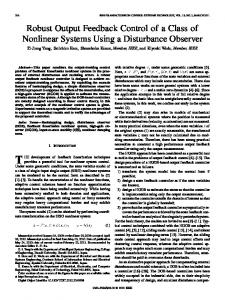
FIG. 1. Plot of the PDF P x (x,t) versus x for ␣ ⫽0.1, ␬ ⫽0.1, x 0 ⫽0.01. The correlation function R(u) has the exponential form R(u)⫽R(0)exp(⫺u/tc) with parameters R(0)⫽0.01 and t c ⫽1. The curves a and b correspond to t⫽0.2 and t⫽0.4, respectively.

which is valid for ␣ ⬍1. Here erf(z)⫽1⫺erfc(z) ⫽(2/冑␲ ) 兰 z0 dt exp(⫺t2) is the error function. According to Eq. 共5.7兲, we have W ⑀ (0)⫽0 if ⑀ ⬍x 0 , W ⑀ (0)⫽1 if ⑀ ⬎x 0 , W ⑀ (⬁)⫽erf„⑀ 1⫺ ␣ / 冑2 ␴ q (⬁)… if ␬ ⬎0, W ⑀ (⬁)⫽0 if ␬ ⫽0 and ␴ q (⬁)⫽⬁, and W ⑀ (t)→0 as ⑀ →0. Specifically, the last condition shows that though P x (0,t)⫽⬁, x⫽0 is indeed not an absorbing point. To summarize, for 0⬍ ␣ ⬍1 the PDF P x (x,t) evolves as follows. If ␬ ⬎0 and 0⬍t⬍t 0 , then P x (x,t) is bimodal 共see Fig. 1, curve a兲. With time, x ⫹ (t) and P x „x ⫹ (t),t… decrease, x ⫺ (t) and P x „x ⫺ (t),t… increase, and at t⫽t 0 the local extrema coalesce. For t⬎t 0 , the PDF P x (x,t) is unimodal 共see Fig. 1, curve b兲, and in the large-time limit it approaches the stationary distribution 共4.18兲. If ␬ ⫽0, then the temporal behavior of P x (x,t) depends on the value of ␴ q (⬁). For ␣) ␴ 2q (⬁)⬍x 2(1⫺ (1⫺ ␣ )/4␣ and t⬎0, the univariate PDF is 0 bimodal as shown in Fig. 1 共curve a兲, and P st (x) is given by ␣) (1⫺ ␣ )/4␣ ⭐ ␴ 2q (⬁)⬍⬁ and t⬍t 0 , Eq. 共4.22兲. For x 2(1⫺ 0 the PDF P x (x,t) is bimodal as shown in Fig. 1 共curve a兲, whereas for t⭓t 0 it is unimodal as shown in Fig. 1 共curve b兲, and P st (x) is given again by Eq. 共4.22兲. Finally, for ␴ q (⬁) ⫽⬁ the PDF P x (x,t) is bimodal for t⬍t 0 and unimodal for t⭓t 0 , but the stationary PDF does not exist and W ⑀ (⬁)⫽0 for any ⑀ . We now consider the case where ␣ ⬍0, i.e., the amplitude of the multiplicative noise diverges as the particle approaches the minimum of the potential well. This is a useful model for exploring situations where the fluctuations drive the system out of the deterministic steady state, whereas the systematic force pushes the system towards it. According to Eq. 共3.21兲, the univariate PDF P x (x,t) has an absolute minimum P x (0,t)⫽0 at x⫽0, P x (x,t)⬃ 兩 x 兩 兩 ␣ 兩 as 兩 x 兩 →0, and Eq. 共5.1兲 has the solutions

that x(t)苸(⫺ ⑀ , ⑀ ). For the power-normal univariate PDF 共3.21兲, Eq. 共5.6兲 leads to the formula

冉

a共 t 兲 ⑀ 1⫺ ␣ 1 ⫹ W ⑀ 共 t 兲 ⫽ erf 2 冑2 冑2 ␴ q 共 t 兲

冉

冊

冊

a共 t 兲 ⑀ 1⫺ ␣ 1 ⫺ ⫺ erf , 2 冑2 冑 2 ␴ q 共 t 兲

共5.7兲

⫾

x 共 t 兲 ⫽⫾x 0 e

⫺␬t

冋 冑 1 ⫾ ⫹ 2

1 ␣ 1 ⫺ 2 4 1⫺ ␣ a 共 t 兲

册

1/共1⫺ ␣ 兲

. 共5.8兲

At x⫽x ⫹ (t), the PDF P x (x,t) has an absolute maximum, P x „x ⫹ (t),t…, and at x⫽x ⫺ (t), it has a local maximum, ” ⬁. Using Eq. P x „x ⫺ (t),t…; P x „x ⫹ (t),t…⬎ P x „x ⫺ (t),t… for t⫽ 共5.8兲, we obtain x ⫹ (t)⬃x ⫹ (t)(t→0) for ␬ ⬎0,

031105-8

STATISTICAL PROPERTIES OF A CLASS OF . . .

冉

x ⫹ 共 t 兲 ⬃x 0 1⫹ for ␬ ⫽0, and x ⫺ 共 t 兲 ⬃⫺

兩␣兩

␴ 2q 共 t 兲

␣) 共 1⫺ ␣ 兲 2 x 2(1⫺ 0

冉

1 兩␣兩 2 ␴ 共t兲 x 0 1⫺ ␣ q

冊

冊

PHYSICAL REVIEW E 65 031105

共 t→0 兲 ,

共5.9兲

共 t→0 兲 ,

共5.10兲

1/共1⫺ ␣ 兲

for ␬ ⭓0, where ␴ 2q (t) is given by Eq. 共4.10兲. In the longtime limit Eq. 共5.8兲 yields x ⫹共 ⬁ 兲 ⫽ 兩 x ⫺共 ⬁ 兲兩 ⫽

冉

兩␣兩 2 ␴ 共⬁兲 1⫺ ␣ q

冊

1/2(1⫺ ␣ )

,

共5.11兲

for ␬ ⬎0, where ␴ 2q (⬁) is defined by Eq. 共4.15兲, and

冉

兩␣兩 2 ␴ 共t兲 x 共 t 兲⬃ 兩 x 共 t 兲兩 ⬃ 1⫺ ␣ q ⫹

⫺

冊

FIG. 2. Plot of the PDF P x (x,t) versus x for ␣ ⫽⫺0.5, ␬ ⫽0.1, x 0 ⫽1, R(0)⫽1, t c ⫽1, and t⫽1 共curve a兲, t⫽5 共curve b兲.

cording to Eq. 共3.22兲, P x (0,t)⫽ P x (⬁,t)⫽0, and P x (x,t) is unimodal for all times. The maximum is located at x ⫽x m (t), x m 共 t 兲 ⫽x 0 exp关 ⫺ ␴ w2 共 t 兲 ⫺ ␬ t 兴 ,

1/2(1⫺ ␣ )

共 t→⬁ 兲 ,

共5.12兲

for ␬ ⫽0 and ␴ q (⬁)⫽⬁, where ␴ 2q (t) is defined by Eq. 共4.19兲. If ␬ ⫽0 and ␴ q (⬁)⬍⬁, Eq. 共5.8兲 yields 兩 x ⫾ (⬁) 兩 ⬍⬁ and x ⫹ (⬁)⬎ 兩 x ⫺ (⬁) 兩 . If ␬ ⬎0 or ␬ ⫽0 and Eq. 共4.20兲 holds, then P x (x,t) approaches the stationary PDF 共4.18兲 or 共4.22兲, respectively, in the long-time limit. If ␬ ⫽0 and Eq. 共4.20兲 does not hold, then 兩 x ⫾ (t) 兩 →⬁ as t→⬁, the stationary PDF does not exist, and W ⑀ (⬁)⫽0 for all ⑀ . In summary, for multiplicative colored Gaussian noise whose amplitude diverges as x→0, the random driving force dominates near x⫽0. It drives the particle away from this point, and the probability density vanishes there. The noise acts symmetrically with respect to x⫽0, which results in temporal bimodality. For ␬ ⬎0, the bimodal behavior of the PDF is stabilized in the long-time limit by the opposing effect of the systematic force, and the system evolves towards a stationary PDF. If the systematic force vanishes, ␬ ⫽0, and the noise intensity of the random force also vanishes, R⫽0, i.e., stochastic localization of free particles occurs, then the bimodal behavior is stabilized by the balance between regions of positive and negative correlations of the noise f (t). Again, the system evolves towards a stationary PDF. If ␬ ⫽0 and the noise intensity is nonzero, then the most probable location of free particles goes to plus or minus infinity as t→⬁, and a stationary PDF does not exist. To illustrate the behavior of the PDF as a function of x, we plot P x (x,t) versus x for different values of ␣ and t in Figs. 2 and 3. The correlation function of the Gaussian noise is again exponential as in Fig. 1. In this case R⫽R(0)t c , and the PDF P x (x,t) approaches the stationary PDF 共4.18兲 as t →⬁. For the case of additive noise, ␣ ⫽0, the univariate PDF is Gaussian according to Eq. 共3.21兲. As before, in this case the function P x (x,t) evolves with time to the stationary PDF 共4.18兲 if ␬ ⬎0, and to the stationary PDF 共4.22兲 if ␬ ⫽0 and F˙ 0 (t)⫽o(1/t) as t→⬁. Otherwise the stationary PDF does not exist. Finally, we consider the case ␣ ⫽1, where the behavior of the PDF near x⫽0 is quite irregular as we will show. Ac-

共5.13兲

and P x „x m 共 t 兲 ,t…⫽

1

冑2 ␲ ␴ w 共 t 兲 x 0

exp关 ␴ w2 共 t 兲 /2⫹ ␬ t 兴 . 共5.14兲

If ␬ ⫽0 and ␴ w (⬁)⬍⬁, then x m (⬁)⫽ ” 0, P x „x m (⬁),⬁…⬍⬁, all fractional moments 共4.9兲 are finite at t⫽⬁, and P x (x,t) approaches the stationary PDF 共4.27兲 as t→⬁. In all other cases we have x m (t)→0 and P x „x m (t),t…→⬁ as t→⬁. Since P x (0,t)⫽0, the long-time behavior of P x (x,t) in a small vicinity of x⫽0 is extremely irregular in those cases. To characterize P x (x,t) near zero, we write the probability W ⑀ (t), using Eqs. 共5.6兲 and 共3.22兲, as W ⑀共 t 兲 ⫽

冉

冊

1 ln共 ⑀ /x 0 兲 ⫹ ␬ t erfc ⫺ . 2 冑2 ␴ w 共 t 兲

共5.15兲

We define

␺ ⫽ lim t→⬁

ln共 ⑀ /x 0 兲 ⫹ ␬ t

冑2 ␴ w 共 t 兲

,

共5.16兲

and taking into account that ␴ w2 (t) grows slower than t 2 , we obtain ␺ ⫽⬁ if ␬ ⬎0, and ␺ ⫽0 if ␬ ⫽0 and R⫽ ” 0. Since erfc (⫺ ␺ )⫽2 in the first case, and erfc (⫺ ␺ )⫽1 in the second case, Eq. 共5.15兲 yields W ⑀ (⬁)⫽1 and W ⑀ (⬁)⫽1/2, re-

FIG. 3. Plot of the PDF P x (x,t) versus x for ␣ ⫽⫺2, ␬ ⫽0.1, x 0 ⫽1, R(0)⫽1, t c ⫽1, and t⫽0.5 共curve a兲, t⫽2 共curve b兲.

031105-9

S. I. DENISOV AND WERNER HORSTHEMKE

PHYSICAL REVIEW E 65 031105

spectively. Though we have x m (⬁)⫽0, P x „x m (⬁),⬁…⫽⬁, and W ⑀ (⬁)⫽1 for ␬ ⬎0, the limit limt→⬁ P x (x,t)⫽ ␦ (x) holds only for R⫽0, when all fractional moments m r (⬁) with r⬎0 equal zero. If R⫽ ” 0, i.e, if regions of positive correlations in the noise dominate, then the long-time behavior of the PDF is determined by the linear random driving force, no matter if a linear systematic restoring force exists, ␬ ⬎0, or not, ␬ ⫽0. The system will not approach a welldefined stationary PDF as t→⬁. In other words, a linear systematic restoring force cannot balance the effects of linear multiplicative colored Gaussian noise, if R⫽ ” 0. The amplitude of the noise must grow slower than 兩 x 兩 as 兩 x 兩 →⬁, if a stationary PDF is to exist for systems of type 共1.1兲. VI. COEFFICIENT OF CORRELATION

In the previous two sections we have characterized the temporal behavior of the Langevin equation 共1.1兲 by studying the single-time PDF and its fractional moments. To obtain further insight into the effects of colored multiplicative Gaussian noise, we now turn our attention to a two-time quantity, the coefficient of correlation, in this section, and a pathwise quantity, the fractal dimension, in the next section. We define the coefficient of correlation of the random process x(t) as usual by R x 共 t,t 1 兲 , r x 共 t,t 1 兲 ⫽ ␴ x共 t 兲 ␴ x共 t 1 兲

r q 共 t,t 1 兲 ⫽

e ⫺ ␻ t 1 F ␻ 共 t 兲 ⫹e ⫺ ␻ t F ␻ 共 t 1 兲 ⫺F ␻ 共 t 1 ⫺t 兲 2 关 e ⫺ ␻ (t⫹t 1 ) F ␻ 共 t 兲 F ␻ 共 t 1 兲兴 1/2

F ␻共 t 兲 ⬃

c␣ t 2⫺ ␤ 共 t→0 兲 , 共 1⫺ ␤ 兲共 2⫺ ␤ 兲

关 ␴ q 共 t 兲 ␴ q 共 t 1 兲兴 1/共1⫺ ␣ 兲 2␲

冕 冕 ⬁

⬁

⫺⬁

⫺⬁

dxdye ⫺(x

which after some algebra leads to the expected result that R x (t,⬁)⫽0 and r x (t,⬁)⫽0, i.e., x(t) and x(⬁) are not correlated for an arbitrary correlation function R(u) and ␬ ⬎0. For free particles, ␬ ⫽0, i.e., ␻ ⫽0, stochastic localization can occur, and we expect the correlation between x(t) and x(t 1 ) to persist for t 1 →⬁. For ␬ ⫽0, Eq. 共6.4兲 is reduced to r q 共 t,t 1 兲 ⫽

F 0 共 t 兲 ⫹F 0 共 t 1 兲 ⫺F 0 共 t 1 ⫺t 兲 2 关 F 0 共 t 兲 F 0 共 t 1 兲兴 1/2

F 0共 z 兲 ⫽

F 0 共 t 1 兲 ⫺F 0 共 t 1 ⫺t 兲 ⫽

共6.2兲

共6.6兲

冕

z

0

共6.7兲

duR 共 u 兲共 z⫺u 兲 .

冕

t1

t 1 ⫺t

duR 共 u 兲共 t 1 ⫺u 兲 ⫹t

冕

t 1 ⫺t

0

duR 共 u 兲 , 共6.8兲

which follows from Eq. 共6.7兲, the formula

冕

t1

t 1 ⫺t

duR 共 u 兲共 t 1 ⫺u 兲 →0 共 t 1 →⬁ 兲 ,

共6.9兲

and the limit ˙ 0 共 t 1 兲 / 冑F 0 共 t 1 兲 ⫽0, lim F

t 1 →⬁

共6.10兲

which for 0⬍R⭐⬁ follows from the conditions F 0 (t 1 ) ⬃t 1 F˙ 0 (t 1 )(t 1 →⬁) and limt 1 →⬁ F˙ 0 (t 1 )/t 1 ⫽0, and for R ⫽0 from F˙ 0 (⬁)⫽R and F 0 (⬁)⬎0, to obtain for finite t,

2 ⫹y 2 )/2

⫻ 兵 关 冑1⫺r 2q 共 t,t 1 兲 y⫹a 共 t 1 兲

r q 共 t,⬁ 兲 ⫽

⫹r q 共 t,t 1 兲 x 兴 兩 冑1⫺r 2q 共 t,t 1 兲 y⫹a 共 t 1 兲 ␣ / 共 1⫺ ␣ 兲

⫺ 关 y⫹a 共 t 1 兲兴 兩 y⫹a 共 t 1 兲 兩 ␣ / 共 1⫺ ␣ 兲 其 .

,

where according to Eq. 共3.9兲 F 0 (z) is defined as

共6.1兲

⫻ 关 x⫹a 共 t 兲兴 兩 x⫹a 共 t 兲 兩 ␣ / 共 1⫺ ␣ 兲

⫹r q 共 t,t 1 兲 x 兩

共6.5兲

We use the relation

is the correlation function, and ␴ 2x (t)⫽R x (t,t) is the dispersion of x(t). Our focus here is the dependence of the limiting value r x (t,⬁) on the noise correlation function R(u). First we consider the case of the power-normal distribution ( ␣ ⬍1). Using Eqs. 共3.13兲 and 共3.21兲 and a transformation of variables, we obtain R x 共 t,t 1 兲 ⫽

共6.4兲

If R(u)⬃c ␣ u ⫺ ␤ 关 0⭐ ␤ ⬍1, c ␣ ⫽R(0) for ␤ ⫽0] as u →0, then for ␻ ⬎0,

where R x 共 t,t 1 兲 ⫽ 具 x 共 t 兲 x 共 t 1 兲 典 ⫺ 具 x 共 t 兲 典具 x 共 t 1 兲 典 ,

.

共6.3兲

Though the integral over y can be expressed by means of the Weber parabolic cylinder functions, we will use Eq. 共6.3兲, which is more suitable for our purposes. According to Eqs. 共3.10兲 and 共3.17兲, the coefficient of correlation r q (t,t 1 ) is given by

1 冑F 共 t 兲 /F 0 共 ⬁ 兲 . 2 0

共6.11兲

According to this formula, r q (t,⬁)⫽0 if t⫽0 or F 0 (⬁) ⫽⬁. The last condition holds if 0⬍R⭐⬁ and also for R ⫽0 if Eq. 共4.20兲 does not hold. In contrast, if the condition 共4.20兲 holds, i.e., stochastic localization of x(t) occurs, then ” 0 and so r x (t,⬁)⫽ ” 0 for t⬎0. This reF 0 (⬁)⬍⬁,r q (t,⬁)⫽ sult shows that correlations between x(t) and x(t⫹t 1 ) exist indeed even for t 1 →⬁ in the case of stochastic localization. Next we consider the case of the lognormal distribution ( ␣ ⫽1). For this case we write the correlation function of x(t) as

031105-10

STATISTICAL PROPERTIES OF A CLASS OF . . .

R x 共 t,t 1 兲 ⫽

PHYSICAL REVIEW E 65 031105

冕冕 ⬁

0

⬁

0

dx dx 1 xx 1 P x 共 x,t;x 1 ,t 1 兲 ⫺m 1 共 t 兲 m 1 共 t 1 兲 .

共6.12兲

Using Eq. 共3.14兲 and introducing the new variables y and y 1 x⫽x 0 e y⫺ ␬ t , x 1 ⫽x 0 e y 1 ⫺ ␬ t 1 ,

共6.13兲

we can reduce Eq. 共6.12兲 to the form R x 共 t,t 1 兲 ⫽

x 20 e ⫺ ␬ (t⫹t 1 )

2 ␲␴ w 共 t 兲 ␴ w 共 t 1 兲 冑1⫺r w2 共 t,t 1 兲 ⫻

冕 冕 ⬁

⫺⬁

⬁

⫺⬁

冋

dy dy 1 exp y⫹y 1 ⫺

1 2 关 1⫺r w2 共 t,t 1 兲兴

冉

y2

␴ w2 共 t 兲

⫹

y 21

⫺

␴ w2 共 t 1 兲

2r w 共 t,t 1 兲 yy ␴ w共 t 兲 ␴ w共 t 1 兲 1

冊册

⫺m 1 共 t 兲 m 1 共 t 1 兲 . 共6.14兲

Performing the integration over y and y 1 in Eq. 共6.14兲 and using Eq. 共4.9兲 and the relation ␴ w2 (t)⫽2F 0 (t), we obtain the explicit formulas for the correlation function R x 共 t,t 1 兲 ⫽m 1 共 t 兲 m 1 共 t 1 兲关 e R w (t,t 1 ) ⫺1 兴

VII. FRACTAL DIMENSION

The fractal dimension d f of a random process x(t) characterizes the irregularity of x(t) and can be defined in various ways 关7,14兴. Here we use the definition 关34兴 ln具 L ␶ 典 , ␶ →0 ln共 1/␶ 兲

⫽x 20 exp关 F 0 共 t 兲 ⫹F 0 共 t 1 兲 ⫺ ␬ 共 t 1 ⫹t 兲兴

d f ⫽1⫹ lim

⫻ 兵 exp关 F 0 共 t 兲 ⫹F 0 共 t 1 兲 ⫺F 0 共 t 1 ⫺t 兲兴 ⫺1 其 , 共6.15兲

where

and for the coefficient of correlation r x 共 t,t 1 兲 ⫽ ⫽

N

具 L ␶ 典 ⫽ 兺 具 冑共 b ␶ 兲 2 ⫹ 关 x 共 t i 兲 ⫺x 共 t i⫺1 兲兴 2 典 ,

e R w (t,t 1 ) ⫺1

exp关 F 0 共 t 兲 ⫹F 0 共 t 1 兲 ⫺F 0 共 t 1 ⫺t 兲兴 ⫺1 关共 e 2F 0 (t) ⫺1 兲共 e 2F 0 (t 1 ) ⫺1 兲兴 1/2

. 共6.16兲

Specifically, if t→0 and R(u)⬃c 1 u ⫺ ␤ (0⭐ ␤ ⬍1) as u →0, then Eqs. 共6.15兲 and 共6.16兲 yield R x (t,t 1 ) ⬃x 0 m 1 (t 1 )F˙ 0 (t 1 )t and

冑

共 1⫺ ␤ 兲共 2⫺ ␤ 兲

2c 1 共 e

2F 0 (t 1 )

⫺1 兲

F˙ 0 共 t 1 兲 t ␤ /2,

共6.17兲

关 c 1 ⫽R(0) for ␤ ⫽0], i.e., R x (0,t 1 )⫽0 (t 1 ⬎0) for all ␤ , whereas r x (0,t 1 )⫽0 only for 0⬍ ␤ ⬍1. According to Eqs. 共6.8兲–共6.10兲, if t 1 ⫽⬁ then

r x 共 t,⬁ 兲 ⫽

共7.2兲

i⫽1

关共 e R w (t,t) ⫺1 兲共 e R w (t 1 ,t 1 ) ⫺1 兲兴 1/2

r x 共 t,t 1 兲 ⬃

共7.1兲

e F 0 (t) ⫺1 关共 e 2F 0 (t) ⫺1 兲共 e 2F 0 (⬁) ⫺1 兲兴 1/2

,

is the average length of x(t) on the interval (t,t⫹⌬t), N ␶ ⫽⌬t, t i ⫽t i⫺1 ⫹ ␶ , t 0 ⫽t, and b is a scaling parameter. In other words, d f characterizes the fractal properties of x(t) on the interval (t,t⫹⌬t). If this interval is small enough, so that the bivariate PDF of x(t) does not change, then Eq. 共7.2兲 is reduced to

具 L ␶典 ⫽

⌬t 具 冑共 b ␶ 兲 2 ⫹ 关 x 共 t⫹ ␶ 兲 ⫺x 共 t 兲兴 2 典 . ␶

共7.3兲

Using Eq. 共3.13兲, we can rewrite Eq. 共7.3兲 for the powernormal distribution in the form

具 L ␶典 ⫽

共6.18兲

if Eq. 共4.20兲 holds, and r x (t,⬁)⫽0 otherwise. Therefore, if ” 0 (t stochastic localization of x(t) occurs, then r x (t,⬁)⫽ ⬎0) for the power-normal as well as the lognormal distributions. 031105-11

⌬t 2␲

冕 冕 ⬁

⬁

⫺⬁

⫺⬁

再

dxdy b 2 ⫹

1

␶2

共 1⫺ ␣ 兲 共 t⫹ ␶ 兲 兵 ␴ 1/ q

⫻ 关 xr q 共 t,t⫹ ␶ 兲 ⫹y 冑1⫺r 2q 共 t,t⫹ ␶ 兲 ⫹a 共 t⫹ ␶ 兲兴 ⫻ 兩 xr q 共 t,t⫹ ␶ 兲 ⫹y 冑1⫺r 2q 共 t,t⫹ ␶ 兲 ⫹a 共 t⫹ ␶ 兲 兩 ␣ /共1⫺ ␣ 兲 共 1⫺ ␣ 兲 ⫺ ␴ 1/ 共 t 兲关 x⫹a 共 t 兲兴 兩 x⫹a 共 t 兲 兩 ␣ /共1⫺ ␣ 兲 其 2 q

⫻e ⫺(x

2 ⫹y 2 )/2

.

冎

1/2

共7.4兲

S. I. DENISOV AND WERNER HORSTHEMKE

PHYSICAL REVIEW E 65 031105

If R(u)⬃c ␣ u ⫺ ␤ (0⭐ ␤ ⬍1) as u→0, then Eqs. 共6.4兲 and 共6.5兲 for ␶ →0 yield 1⫺r 2q (t,t⫹ ␶ )⬀ ␶ 2⫺ ␤ , and Eq. 共7.4兲 leads to 具 L ␶ 典 ⬀ ␶ ⫺ ␤ /2. As a consequence, we obtain from Eq. 共7.1兲

VIII. CONCLUSIONS

Since 1⫺r w2 (t,t⫹ ␶ )⬀ ␶ 2⫺ ␤ for ␶ →0, Eq. 共7.6兲 yields 具 L ␶ 典 ⬀ ␶ ⫺ ␤ /2, and the fractal dimension of random processes with a lognormal distribution is given by the same formula 共7.5兲 as for the power-normal distribution.

We have studied the statistical properties of nonlinear systems driven by colored Gaussian noise whose amplitude depends on a power of the system state, 兩 x 兩 ␣ . Starting from the exact solution x(t) of the Langevin equation, we have obtained the univariate and bivariate PDFs of x(t) and shown that, depending on the exponent ␣ , the solution is described by the lognormal 共if ␣ ⫽1) or the power-normal 共if ␣ ⬍1) distribution. We have found that in both cases the system can exhibit the phenomenon of stochastic localization, i.e., a stationary univariate PDF for free particles exists, and we have derived the criterion when this occurs. We have studied in detail the time evolution of the univariate PDF, found exact expressions for the fractional moments of x(t), and obtained and analyzed their short- and long-time asymptotics. Specifically, the long-time behavior of the dispersion of the particle position shows that diffusion of free particles can have anomalous character, and we have determined the conditions that lead to subdiffusion and superdiffusion. Using the bivariate PDF, we have obtained an integral representation for the correlation function R x (t,t 1 ) and for the coefficient of correlation r x (t,t 1 ) of x(t) for ␣ ⬍1, and for ␣ ⫽1 we have expressed R x (t,t 1 ) and r x (t,t 1 ) in terms of elementary functions. We have shown that if stochastic localization occurs, then x(t) and x(t⫹t 1 ) are correlated even as t 1 →⬁, i.e., in the case of stochastic localization the con” 0 (t⬎0) holds, and r x (t,⬁)⫽0 in all other dition r x (t,⬁)⫽ cases. Also, we have calculated the fractal dimension d f of x(t) and established that x(t) is fractal, i.e., d f ⬎1, if the noise correlation function R(u) has a power singularity at u⫽0.

关1兴 J. Martı´n-Regaldo, S. Balle, and N. B. Abraham, IEEE J. Quantum Electron. 32, 257 共1996兲. 关2兴 D. Ludwig, Stochastic Population Theories, Lecture Notes in Biomathematics Vol. 3 共Springer, Berlin, 1978兲. 关3兴 T. Maruyama, Stochastic Problems in Population Genetics, Lecture Notes in Biomathematics Vol. 17 共Springer, Berlin, 1977兲. 关4兴 H. C. Tuckwell, Stochastic Processes in the Neurosciences 共SIAM, Philadelphia, 1989兲. 关5兴 W. Horsthemke and R. Lefever, Noise-Induced Transitions 共Springer-Verlag, Berlin, 1984兲. 关6兴 J. Garcı´a-Ojalvo and J. M. Sancho, Noise in Spatially Extended Systems 共Springer-Verlag, New York, 1999兲. 关7兴 A.-L. Baraba´si and H. E. Stanley, Fractal Concepts in Surface Growth 共Cambridge University Press, Cambridge, England, 1995兲. 关8兴 H. K. Janssen, Z. Phys. B: Condens. Matter 42, 151 共1981兲. 关9兴 P. Grassberger, Z. Phys. B: Condens. Matter 47, 365 共1982兲. ˜ oz, Phys. Rev. E 57, 1377 共1998兲. 关10兴 M. A. Mun 关11兴 G. P. Saracco and E. V. Albano, Phys. Rev. E 63, 036119 共2001兲. 关12兴 J. Y. Campbell, A. Lo, and A. C. MacKinlay, The Econometrics of Financial Markets 共Princeton University Press, Princeton, 1997兲. 关13兴 M. Levy and S. Solomon, Int. J. Mod. Phys. C 7, 595 共1996兲;

H. Takayasu, A.-H. Sato, and M. Takayasu, Phys. Rev. Lett. 79, 966 共1997兲; D. Sornette, Phys. Rev. E 57, 4811 共1998兲; H. Nakao, ibid. 58, 1591 共1998兲; S. C. Manrubia and D. H. Zanette, ibid. 59, 4945 共1999兲; A.-H. Sato, H. Takayasu, and Y. Sawada, ibid. 61, 1081 共2000兲. B. B. Mandelbrot, The Fractal Geometry of Nature 共Freeman, New York, 1982兲. P. Bak, How Nature Works 共Oxford University Press, Oxford, 1997兲. J. L. Doob, Stochastic Processes 共Wiley, New York, 1953兲. C. W. Gardiner, Handbook of Stochastic Methods, 2nd ed. 共Springer-Verlag, Berlin, 1990兲. H. Risken, The Fokker-Planck Equation, 2nd ed. 共SpringerVerlag, Berlin, 1990兲. M. Magnasco, Phys. Rev. Lett. 71, 1477 共1993兲; R. D. Astumian and M. Bier, ibid. 72, 1766 共1994兲; C. R. Doering, W. Horsthemke, and J. Riordan, ibid. 72, 2984 共1994兲; R. Bartussek, P. Reimann, and P. Ha¨nggi, ibid. 76, 1166 共1996兲; R. D. Astumian, Science 276, 917 共1997兲; J. M. R. Parrondo, Phys. Rev. E 57, 7297 共1998兲; E. Corte´s, Physica A 275, 78 共2000兲; M. N. Popescu, C. M. Arizmendi, A. L. Salas-Brito, and F. Family, Phys. Rev. Lett. 85, 3321 共2000兲. J. Masoliver, Phys. Rev. A 45, 706 共1992兲; J. Heinrichs, Phys. Rev. E 47, 3007 共1993兲; J. Masoliver and K. G. Wang, ibid. 51, 2987 共1995兲.

d f ⫽1⫹ ␤ /2.

共7.5兲

This result shows that the random processes with a powernormal distribution considered here have fractal properties only if 0⬍ ␤ ⬍1, i.e., only if the noise correlation function R(u) has a singularity at u⫽0. Note also that for such processes the fractal dimension d f does not depend on t. In the case of the lognormal distribution, Eq. 共7.3兲 can be written as ⌬t 具 L ␶典 ⫽ 2␲

冕 冕 ⬁

⬁

⫺⬁

⫺⬁

再

dxdy b ⫹ 2

x 20

␶2

兵 exp关 x ␴ w 共 t 兲 ⫺ ␬ t 兴

⫺exp关 y ␴ w 共 t⫹ ␶ 兲 冑1⫺r w2 共 t,t⫹ ␶ 兲 ⫺ ␬ 共 t⫹ ␶ 兲 ⫹x ␴ w 共 t⫹ ␶ 兲 r w 共 t,t⫹ ␶ 兲兴 其

2

冎

1/2

e ⫺(x

2 ⫹y 2 )/2

.

共7.6兲

关14兴 关15兴 关16兴 关17兴 关18兴 关19兴

关20兴

031105-12

STATISTICAL PROPERTIES OF A CLASS OF . . .

PHYSICAL REVIEW E 65 031105

关21兴 R. Muralidhar, D. Ramkrishna, H. Nakanishi, and D. Jacobs, Physica A 167, 539 共1990兲; K. G. Wang, Phys. Rev. A 45, 833 共1992兲; J. M. Porra´, K. G. Wang, and J. Masoliver, Phys. Rev. E 53, 5872 共1996兲; K. G. Wang and M. Tokuyama, Physica A 265, 341 共1999兲. 关22兴 F. Lillo and R. N. Mantegna, Phys. Rev. E 61, R4675 共2000兲. 关23兴 S. I. Denisov and W. Horsthemke, Phys. Rev. E 62, 7729 共2000兲. 关24兴 S. I. Denisov and W. Horsthemke, Phys. Lett. A 282, 367 共2001兲. 关25兴 N. G. Van Kampen, Stochastic Processes in Physics and Chemistry 共North-Holland, Amsterdam, 1992兲. 关26兴 J. Aitcheson and J. A. C. Brown, The Log-Normal Distribution 共Cambridge University Press, London, 1957兲.

关27兴 S. I. Denisov and W. Horsthemke 共unpublished兲. 关28兴 W. Feller, An Introduction to Probability Theory and its Applications, 2nd ed. 共Wiley, New York, 1971兲, Vol. 2. 关29兴 W. Feller, An Introduction to Probability Theory and its Applications, 3rd ed. 共Wiley, New York, 1968兲, Vol. 1. 关30兴 R. L. Stratonovich, SIAM J. Control 4, 362 共1966兲. 关31兴 Handbook of Mathematical Functions, 9th ed., edited by M. Abramowitz and I. A. Stegun 共Dover, New York, 1972兲. 关32兴 H. Bateman and A. Erde´lyi, Higher Transcendental Functions 共McGraw-Hill, New York, 1953兲, Vol. 2. 关33兴 F. W. J. Olver, Introduction to Asymptotics and Special Functions 共Academic Press, New York, 1974兲. 关34兴 S. I. Denisov, Chaos, Solitons Fractals 9, 1491 共1998兲.

031105-13