Stiction Detection and Quantification as an

Stiction Detection and Quantification as an Application of Optimization Ana S.R. Br´ asio1,2, Andrey Romanenko2 , and Nat´ercia C.P. Fernandes1 1

CIEPQPF, Department of Chemical Engineering University of Coimbra, Portugal {anabrasio,natercia}@eq.uc.pt 2 Ciengis, SA, Coimbra, Portugal [email protected]

Abstract. Stiction is a major problematic phenomenon affecting industrial control valves. An approach for detection and quantification of valve stiction using an one-stage optimization technique is proposed. A Hammerstein Model that comprises a complete stiction model and a process model is identified from industrial process data. Some difficulties in the identification approach are pointed out and strategies to overcome them are suggested, namely the smoothing of discontinuity points. A simulation study demonstrates the application of the proposed technique. Keywords: system identification, non-linear optimization, smoothing discontinuous functions, stiction detection and quantification.

1

Introduction

Stiction is one of the long-standing control valve problems in the process industry causing oscillations and, consequently, losses of productivity. Therefore, it is important to understand this phenomenon for its early detection and separation from other oscillation causes. Because stiction is one of the major causes for oscillations in the controlled variable, numerous techniques for its detection and quantification in linear control loops have been suggested. Recently, stiction detection and quantification developments were proposed by means of system identification using the Hammerstein Model [1–11]. System identification deals with the building of mathematical models to describe dynamical systems based on observed data [12]. The use of optimization techniques for system identification has become more common, motivated by successful applications in different areas [13]. The Hammerstein Model is a model that consists of a static non-linear element in series with a linear dynamic part [14]. In the context of an industrial control loop, the non-linear element represents the sticky valve while the linear part models the process dynamics, as shown in Fig. 1. One of the identification strategies for such models is the decoupling of the non-linear and linear parts [2, 5, 11], with the process model parameters determined in the first place followed by the determination of the stiction model parameters. B. Murgante et al. (Eds.): ICCSA 2014, Part II, LNCS 8580, pp. 169–179, 2014. c Springer International Publishing Switzerland 2014 ⃝

170

A.S.R. Br´ asio, A. Romanenko, and N.C.P. Fernandes

Fig. 1. Industrial control loop representing the Hammerstein Model, where ysp is the variable setpoint, u is the controller output, x is the real valve position, and y is the controlled variable

The modeling of stiction may be carried out using first-principle or datadriven models. Data-driven models [1, 15–21] have been used more frequently due to their reduced number of parameters, simplicity and easy computational implementation. ARX [1, 2], ARMAX [6] models, or transfer functions [3] are examples of data-driven approaches. However, these models contain discontinuities in their formulation which is a significant disadvantage. The present work explores the application of continuous optimization techniques to the system identification of a model with the stiction phenomenon. A strategy to deal with the discontinuities of the used Hammerstein Model in the context of the optimization procedure is proposed. The paper is organized as follows: in Section 2, the proposed method is presented; Section 3 details a smoothing approach to avoid model discontinuities; in Section 4, the results are shown and discussed and, finally, in Section 5, main conclusions are drawn.

2

Method Formulation

A novel technique for detection and quantification of valve stiction in control loops based on one-stage identification is proposed in this section. The system to be identified is represented by the Hammerstein Model shown in Fig. 1. After sufficiently rich process data is collected, the model parameters are determined such that the model response reproduces the observed response of the actual process. Mathematically, this is represented by the non-linear constrained optimization problem minimize

J(y, u, p)

(1a)

subject to

y˙ = f (y, x, p) x = g(u, p)

(1b) (1c)

yL ≤ y ≤ yU

(1d)

h(p) ≤ 0,

(1g)

p

uL ≤ u ≤ uU pL ≤ p ≤ pU

(1e) (1f)

Stiction Detection and Quantification

171

where J denotes the objective function, p is the parameters vector including both the stiction and the process models, y and u are the vectors of controlled variable and controller output (respectively), x is the vector of the real valve position, and the subscripts L and U stand for lower and upper bounds (respectively). The set of equations (1b) and (1c) defines a set of constraints arising from the Hammerstein Model dynamics. Inequalities (1g) enforce additional identification criteria. As it may be seen in Fig. 1, the non-linear element scales the controller output and transforms it to the real valve position. The model expressed by the set of equations (1b) corresponds to this transformation and is represented by a stiction model existent in the literature. In contrast, the linear element whose output is the controlled variable is modeled by the linear model specified by (1c). Given the Hammerstein Model and a set of n experimental data points (ti , yexp,i ), the objective function J is written, according to the minimum least squares criterion, as "⊤ ! " ! J = yexp − y Q yexp − y ,

(2)

where Q is a diagonal matrix containing the weights given to each observed variable. In this work, equal weight was given to all output variables. From a practical point of view, the proposed technique only requires the controller output and the controlled variable data that may be accessed in the DCS (Distributed Control System) of industrial plants. Notice that the real valve position is an unmeasured intermediate variable.

3

Smoothing of Discontinuous Models

Stiction is essentially described by discontinuous non-linear models and that calls for mixed integer non-linear optimization problem formulation and a special class of optimizers. Alternatively, smoothing approaches for discontinuous models have been successfully applied. Some works introduced smoothing techniques in the context of exact penalty functions [22–24]. Others authors have suggested to express discontinuities by means of a step function and then to substitute this function by a continuous approximation [25–27]. This is the approach also adopted in the present work. Consider the general discontinuous system ⎧ z1 (t), if t ∈ T1 ⎪ ⎪ ⎪ ⎨ z2 (t), if t ∈ T2 , (3) z(t) = . .. ⎪ ⎪ ⎪ ⎩ zm (t), if t ∈ Tm

where zi (t), i = 1, · · · , m, are continuously differentiable real functions over Rn subject to the conditions that define the subsets Ti . Assuming that the real

172

A.S.R. Br´ asio, A. Romanenko, and N.C.P. Fernandes

expressions ek (t), k = 1, · · · , p, are continuously differentiable over Rn , the subsets Ti are defined as Ti = {t ∈ Rn : ek (t) < 0, ∀k ∈ Li ; ek (t) ≥ 0, ∀k ∈ Gi } ,

(4)

where Li and Gi are, for branch i, the sets of indexes k for which ek (t) < 0 and ek (t) ≥ 0, respectively. The discontinuous function (3) may be expressed by means of the Heaviside function as m " " ! z(t) = [1 − H(ek )] H(ek ) zi (t) , (5) i=1 k∈Li

with

k∈Gi

H(t) =

#

1, 0,

if t ≥ 0 , if t < 0

(6)

H(ek ) =

#

1, 0,

if ek ≥ 0 . if ek < 0

(7)

that is,

It is possible to smooth the Heaviside function by approximating it by the hyperbolic function %& $ t = 0.5 + 0.5 · tanh (r · t) , H (8) %& $ t is second-order continuously differentiable on Rn varying within the where H interval [0, 1], and r is an accuracy parameter. Similarly to the approach of [27], the step function approximation here considered contains a single parameter. This parameter controls the accuracy of the approximation by adjusting the size of the neighborhoods around the discontinuity points over which the approximation has an effective effect. Therefore, the continuous differentiable on Rn function that approximates function (3) may be written as z$(t) =

4

m " ' ( " ! $ k) $ k ) zi (t) . H(e 1 − H(e i=1 k∈Li

(9)

k∈Gi

Application to a System Containing a Sticky Valve

As mentioned above, the Hammerstein Model comprises a non-linear model describing the sticky valve and a linear process model. The present paper uses the complete Chen Model, also called by the authors as two-layer binary tree model [18], to model the sticky valve. In what concerns the process dynamics, it is modeled by the single-input single-output state-space model y˙ ∗ = a y∗ + b x∗ ,

(10)

Stiction Detection and Quantification

173

where a and b are state-space model constants, and the deviation variables vectors y∗ and x∗ are related to the original variables y and x through the simple translations y∗ = y − y¯ and x∗ = x − x ¯, respectively. In order to collect experimental data needed to perform a comparison between the smoothed and the original versions of the Chen Model and also needed for the identification process, a plant simulation was carried out using the Hammerstein Model containing the original discontinuous Chen Model. The parameters used in the simulation are: (i) for the stiction model: fS = 2.8 % and fD = 0.9 %; ¯ = 0 %. A sinusoidal (ii) for the process model: a = 1, b = −1 %−1 , y¯ = 0, and x excitation on the controller output with amplitude of 5 % and period of 40 min is applied to the system to generate a response, yexp , that includes sufficient dynamical information about the valve and the process. The obtained dataset contains n = 101 points covering an interval of 50 minutes with a sampling period of 0.5 minutes.

4.1

Smoothing of the Stiction Model

An enhanced flow diagram of the Chen Model is illustrated in Fig. 2. The diagram is complemented with some notes, relatively to the original model presented by its authors in [18], to better explain the model and the approach developed in the present paper.

Fig. 2. Enhanced Chen Model flow diagram

174

A.S.R. Br´ asio, A. Romanenko, and N.C.P. Fernandes

The Chen Model may be rewritten as ⎧ z1 (t), if e1 (t) = 1 ∧ e2 (t) ≥ 0 ⎪ ⎪ ⎨ z2 (t), if e1 (t) = 1 ∧ e2 (t) < 0 , z(t) = z3 (t), if e1 (t) = 0 ∧ e3 (t) < 0 ⎪ ⎪ ⎩ z4 (t), if e1 (t) = 0 ∧ e3 (t) ≥ 0

(11)

where z(t) is a general variable used to represent the outputs c(t), x(t) and s(t). Expressions e1 (t) and e2 (t) are given by e1 (t) = s(t − 1) ,

e2 (t) = c(t) − fS ,

(12) (13)

where s(t) is the valve status flag, c(t) is the accumulated force compensated by friction, and fS is a model constant. The expression e3 (t) becomes positive or equal to zero when % & % & e31 (t) ≥ 0 ∧ e32 (t) ≥ 0 ∨ e31 (t) < 0 ∧ e33 (t) ≥ 0 , (14) with

e31 (t) = fD ,

(15)

e32 (t) = |c(t)| − fD , e33 (t) = d(t) · d(t − 1) ,

(16) (17)

where d(t) is the movement direction, and fD is a model constant. Notice that the condition fD < 0 ∧ |c(t)| < −fD (see decision diamond-shaped box e3 (t) of Fig. 2) is not considered in the formulation, because it is assumed that fD ≥ 0. The expression e3 (t) becomes negative otherwise. The Chen Model contains m = 4 branches subject to p = 3 conditions. Sets Li and Gi are defined as L1 = {}, L2 = {2}, L3 = {1, 3}, L4 = {1} , G4 = {3} . G1 = {1, 2}, G2 = {1}, G3 = {}, The continuous and differentiable function that approximates (11) is therefore defined by * ( ) ( )+ ' e2 · z1 (t) + ' e2 · e1 (t) · z2 (t) z'(t) = e1 (t) · H 1−H * ( )+ ( ) ' e3 · z3 (t) + [1 − e1 (t)] · H ' e3 · z4 (t) , (18) + [1 − e1 (t)] · 1 − H with

( ) ( ) ( ) * ( )+ ( ) ' e3 = H ' e31 · H ' e32 + 1 − H ' e31 · H ' e33 . H

(19)

Stiction Detection and Quantification

175

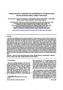
It is noteworthy that e1 (t) is used in (11) inside an equality condition which precludes the direct usage of the approximation approach described in Section 3. However, as shown in (12), this condition is given by the output s(t − 1) which is ! smoothed and valued between 0 and 1 similarly to H(t). These facts enable the use of this variable directly in equation (18) in a similar way as the smoothed Heaviside functions, allowing to deal with the equality constraint. Several simulations were performed in order to assess the performance of the developed approach. Fig. 3 depicts the simulation responses of the Hammerstein Model when the non-linear element is described by the original Chen Model (solid line) and also when the non-linear element is described by the smoothed Chen Model, proposed in the present paper (dashed lines and points). Being a measure of the quality of the approximation applied, the parameter r has a visible influence on the performance of the smoothed model. This influence is quantified in Table 1 by the mean squared error (MSE) associated with the simulations for different values of r. As it may be easily seen in Fig. 3, by using bigger values of r it is possible to reproduce better the data obtained by the original Chen Model. For bigger values of r, the approximation of the function occurs in smaller neighborhoods of the discontinuity points leading to a better

original r = 0.05 r = 0.5 r=5 r = 50

5.0

y∗ , –

2.5

0.0

-2.5

-5.0 0

10

20

30

40

50

t, min

Fig. 3. Comparison between the Hammerstein Model using the original Chen Model and its smoothed version for different values of r Table 1. MSE for different values of r r MSE

0.05

0.5

5

10

20

30

40

50

88.440

34.459

39.701

0.829

0.011

0.003

0.002

0.000

176

A.S.R. Br´ asio, A. Romanenko, and N.C.P. Fernandes

approximation. The value of r = 50 was selected based on a mean squared error tolerance of 10−3 . 4.2

Stiction Detection and Quantification

The Chen Model parameter fS is linearly dependent on fD through the mathematical relationship [18] (20) fS = fD + fJ . Such dependence poses a difficulty in system identification, because it compromises the identifiability of the individual parameters. In order to overcome this problem, the model is reformulated to use parameters fJ instead of fS for optimization purposes. Table 2. System identification results

p

Initial

pL

pU

Fit

Indicators

a, – b, % y¯, – x ¯, %−1 fJ , % fD , %

-0.200 0.020 1.000 1.000 0.000 0.000

-10 -10 -10 -10 0 0

10 10 10 10 10 10

-0.998 0.998 0.000 0.000 1.732 0.898

J = 0.001 R2 = 1.000

Q = 102 I101 , where In is the identity matrix of size n × n.

The optimization procedure described in Section 2 was used to identify the system. The implementation was made in GNU Octave 3.6.3 using its general non-linear sqp() (successive quadratic programming) solver. The set of optimization related conditions and the obtained model parameters as well as some fitting quality indicators are presented in Table 2. The optimization tolerance was 10−20 . In order to avoid poor ! conditioning of " the data, the parameters were normalized by the vector α = −0.1 0.1 1 1 1 1 , with the necessary changes in the model. ∗ , may be directly compared The profile predicted by the identified model, yfit ∗ ∗ with the experimental profile, yexp , in Fig. 4. The initial profiles, yinit and x∗init , are also displayed revealing that the starting initial situation was significantly different from the experimental profiles. As it is possible to observe, the fitted Hammerstein Model is able to capture well the sticky valve and the process dynamics. The high correlation factor, R2 , and the lower objective function prove the effectiveness of the one-stage system identification technique.

Stiction Detection and Quantification

177

y∗exp y∗init y∗fit

5.0

y∗ , –

2.5 0.0 -2.5 -5.0

0

10

20

30

40

50

t, min uexp x∗init x∗fit

5.0

∗

u and x , %

2.5 0.0 -2.5 -5.0

0

10

20

30

40

50

t, min

Fig. 4. System identification

5

Conclusions

A technique for detection and quantification of valve stiction in control loops based on one-stage optimization technique was developed using the Sequential Quadratic Programming algorithm. The modeling approach adopted to describe a process containing a sticky valve is the so-called Hammerstein Model, which includes a non-linear element in series with a linear element. The former corresponds to the sticky valve and is modeled according to the Chen Model. The latter represents the process and is modeled by a single-input single-output state-space model. Because the Chen Model discontinuities originate system identification difficulties, an approach based on the discontinuity points smoothing was suggested and successfully applied to the model. Finally, the smoothed Hammerstein Model

178

A.S.R. Br´ asio, A. Romanenko, and N.C.P. Fernandes

identified using the one-stage optimization technique reproduced quite well the experimental data. Acknowledgments. This work was developed under project NAMPI, reference 2012/023007, in consortium between Ciengis, SA and the University of Coimbra, with financial support of QREN via Mais Centro operational regional program and European Union via FEDER framework program. The authors also acknowledge CIEPQPF for providing conditions to develop and present this work.

References 1. Stenman, A., Gustafsson, F., Forsman, K.: A segmentation-based method for detection of stiction in control valves. Int. J. Adapt. Control 17(7-9), 625–634 (2003) 2. Srinivasan, R., Rengaswamy, R., Narasimhan, S., Miller, R.: Control loop performance assessment. 2. Hammerstein model approach for stiction diagnosis. Ind. Eng. Chem. Res. 44(17), 6719–6728 (2005) 3. Lee, K., Ren, Z., Huang, B.: Novel closed-loop stiction detection and quantification method via system identification. In: International Symposium on Advanced Control of Industrial Processes (2008) 4. Choudhury, S., Jain, M., Shah, S.L.: Stiction – Definition, modelling, detection and quantification. J. Process Contr. 18, 232–243 (2008) 5. Jelali, M.: Estimation of valve stiction in control loops using separable least-squares and global search algorithms. J. Process Contr. 18(7-8), 632–642 (2008) 6. Ivan, L., Lakshminarayanan, S.: A new unified approach to valve stiction quantification and compensation. Ind. Eng. Chem. Res. 48(7), 3474–3483 (2009) 7. Karra, S., Karim, M.: Comprehensive methodology for detection and diagnosis of oscillatory control loops. Control Eng. Pract. 17(8), 939–956 (2009) 8. Lee, K., Tamayo, E., Huang, B.: Industrial implementation of controller performance analysis technology. Control Eng. Pract. 18(2), 147–158 (2010) 9. Qi, F., Huang, B.: Estimation of distribution function for control valve stiction estimation. J. Process Contr. 21(8), 1208–1216 (2011) 10. Srinivasan, B., Spinner, T., Rengaswamy, R.: A reliability measure for model based stiction detection approaches. In: Symposium on Advanced Control of Chemical Processes, pp. 750–755 (2012) 11. Babji, S., Nallasivam, U., Rengaswamy, R.: Root cause analysis of linear closedloop oscillatory chemical process systems. Ind. Eng. Chem. Res. 51(42), 13712– 13731 (2012) 12. Ljung, L.: System identification: theory for the user. Prentice-Hall, New Jersey (1999) 13. Vandenberghe, L.: Convex optimization techniques in system identification. Technical report, University of California (2014) 14. Eskinat, E., Johnson, S., Luyben, W.: Use of Hammerstein models in identification of nonlinear systems. AIChE J. 37(2), 255–268 (1991) 15. Choudhury, A., Thornhill, N., Shah, S.: Modelling valve stiction. Control Eng. Pract. 13(5), 641–658 (2005) 16. Kano, M., Maruta, H., Kugemoto, H., Shimizu, K.: Practical model and detection algorithm for valve stiction. In: IFAC Symposium on Dynamics and Control of Process Systems, pp. 859–864. Elsevier, United Kingdom (2004)

Stiction Detection and Quantification

179

17. He, Q., Wang, J., Pottmann, M., Qin, J.: A curve fitting method for detecting valve stiction in oscillating control loops. Ind. Eng. Chem. Res. 46(13), 4549–4560 (2007) 18. Chen, S., Tan, K., Huang, S.: Two-layer binary tree data-driven model for valve stiction. Ind. Eng. Chem. Res. 47(8), 2842–2848 (2008) 19. Zabiri, H., Mazuki, N.: A black-box approach in modeling valve stiction. J. Eng. Appl. Sci. 6(5), 277–284 (2010) 20. Wang, J., Sano, A., Chen, T., Huang, B.: A blind approach to identification of Hammerstein systems. In: IFAC World Congress on Block-oriented Nonlinear System Identification, pp. 293–312. Springer, London (2010) 21. Karthiga, D., Kalaivani, S.: A new stiction compensation method in pneumatic control valves. Int. J. Electron. Comput. Sci. Eng., 2604–2612 (2012) 22. Wu, Z., Bai, F., Yang, X., Zhang, L.: An exact lower order penalty function and its smoothing in nonlinear programming. Optimization 53(1), 51–68 (2004) 23. Wu, Z., Lee, H., Bai, F., Zhang, L.: Quadratic smoothing approximation to l1 exact penalty function in global optimization. J. Ind. Manag. Optim. 1(4), 533– 547 (2005) 24. Meng, K., Li, S., Yang, X.: A robust SQP method based on a smoothing lower order penalty function. Optimization 58(1), 23–38 (2009) 25. Goldfeld, S., Quandt, R.: Nonlinear methods in econometrics. North-Holland Publishing Company (1972) 26. Tishler, A., Zang, I.: A switching regression method using inequality conditions. J. of Econometrics 11(2-3), 259–274 (1979) 27. Zang, I.: Discontinuous optimization by smoothing. Math. Oper. Res. 6(1), 140–152 (1981)