J. lnf. Commun. Converg. Eng. 11(2): 95-102, Jun. 2013
Regular paper
Stochastic Mixture Modeling of Driving Behavior During Car Following Pongtep Angkititrakul*, Chiyomi Miyajima, and Kazuya Takeda, Member, KIICE Department of Media Science, Graduate School of Information Science, Nagoya University, Nagoya 464-8603, Japan
Abstract This paper presents a stochastic driver behavior modeling framework which takes into account both individual and general driving characteristics as one aggregate model. Patterns of individual driving styles are modeled using a Dirichlet process mixture model, as a non-parametric Bayesian approach which automatically selects the optimal number of model components to fit sparse observations of each particular driver’s behavior. In addition, general or background driving patterns are also captured with a Gaussian mixture model using a reasonably large amount of development data from several drivers. By combining both probability distributions, the aggregate driver-dependent model can better emphasize driving characteristics of each particular driver, while also backing off to exploit general driving behavior in cases of unseen/unmatched parameter spaces from individual training observations. The proposed driver behavior model was employed to anticipate pedal operation behavior during car-following maneuvers involving several drivers on the road. The experimental results showed advantages of the combined model over the model adaptation approach.
Index Terms: Car following, Driver behavior, Mixture model, Model adaptation, Non-parametric Bayesian each having different characteristics and corresponding parameters. Therefore, complex driving behavior can be broken down into a reasonable number of sub-patterns. For instance, during car following, it is believed that drivers adopt different driving patterns or driving modes (e.g., normal following, approaching) under different driving situations, depending on individual and contextual factors. One challenge in behavior modeling is to determine how many latent classes or localized relationships exist between the stimuli and the driver’s responses (i.e., model selection problem), and to estimate the properties of these hidden components from the given observations. In general, a trade-off in selecting the number of components arises: with too many components, the obtained model may over-fit the data, while a model with too few components may not be flexible enough to represent an underlying distribution of observations.
I. INTRODUCTION Predicting driving behavior by employing mathematical driver models, which are obtained directly from the observed driving-behavior data, has gained much attention in recent research. Various approaches have been proposed for modeling driving behavior based on different interpretations and assumptions, such as the piecewise autoregressive exogenous (PWARX) model [1, 2], hidden Markov model (HMM) [3], neural network (NN) [4], and Gaussian mixture model (GMM) [5]. These approaches have reported impressive performance on simulated and controlled driving data. Some of these promising techniques exploit a set of localized relationships to model driving behavior (e.g., mixture models, piecewise linear models). These models assume that the observed data are generated by a set of latent components,
___________________________________________________________________________________________ Received 28 December 2012, Revised 15 January 2013, Accepted 02 February 2013 *Corresponding Author Pongtep Angkititrakul (E-mail:
[email protected];
[email protected], Tel: +81-52-789-3647) Department of Media Science, Graduate School of Information Science, Nagoya University, Furo-cho, Chikusa-ku, Nagoya 464-8603, Japan. Open Access
http://dx.doi.org/10.6109/jicce.2013.11.2.095
print ISSN: 2234-8255 online ISSN: 2234-8883
This is an Open Access article distributed under the terms of the Creative Commons Attribution Non-Commercial License (http://creativecommons.org/li-censes/bync/3.0/) which permits unrestricted non-commercial use, distribution, and reproduction in any medium, provided the original work is properly cited. Copyright ⓒ The Korea Institute of Information and Communication Engineering
95
J. lnf. Commun. Converg. Eng. 11(2): 95-102, Jun. 2013
individual driver behavior model in order to capture unique driving styles from available observations. Furthermore, in order to cope with unseen or unmatched driving situations that may not be present in individual training observations, we employed a GMM with a classical EM algorithm to train a universal driver model from observations of several drivers. Finally, the driver-dependent model is obtained by combining both driver models into one aggregate model in a probabilistic manner. As a result, the combined model contains both individual and background distributions that can better represent both observed and unobserved driving behavior of individual drivers. Experimental validation was conducted by observing the car-following behavior of several drivers on the road. The objective of a driver behavior model is to anticipate carfollowing behavior in terms of pedal control operations (i.e., gas and brake pedal pressures) in response to the observable driving signals, such as the vehicle velocity and the following distance behind the leading vehicle. We demonstrated that the proposed combined driver model showed better prediction performance than both individual and general models, as well as the driver-adapted model based on the maximum a posteriori (MAP) criterion [5].
A finite GMM [6] is a well-known probabilistic and unsupervised modeling technique for multivariate data with an arbitrarily complex probability density function (pdf). Expectation-maximization (EM) is a powerful algorithm for estimating parameters of finite mixture models that maximizes the likelihood of observed data. However, the EM algorithm is sensitive to initialization (i.e., it may converge to a local maximum), and may converge to the boundary of a parameter space, leading to a meaningless estimate [6]. Moreover, EM provides no explicit solution to the model selection problem, and may not yield a wellbehaved distribution when the amount of training data is insufficient. Recently, the Dirichlet process mixture model (DPM), a non-parametric Bayesian approach, has been proposed to circumvent such issues [7, 8]. Unlike finite mixture models, DPM estimates the joint distribution of stimuli and responses using a Dirichlet process mixture by assuming that the number of components is random and unknown. Specifically, a hidden parameter is first drawn from a base distribution; consequently, observations are generated from a parametric distribution conditioned on the drawn parameter. Therefore, DPM avoids the problem of model selection by assuming that there are an infinite number of latent components, but that only a finite number of observations could be observed. Most importantly, DPM is capable of choosing an appropriate number of latent components to explain the given data in a probabilistic manner. DPM has been successfully applied in several applications such as modeling content of documents and spike sorting [7, 9]. In car following, driver behavior is influenced by both individual and situational factors [10, 11]; hence, the best driver behavior model for each particular driver should be obtained by using individual observations that include all possible driving situations. However, at present, it is not practical to collect such a large amount of driving data from one particular driver in order to create a driver-specific model. To circumvent this issue, a general or universal driver model, which is obtained by using a reasonable amount of observations from several drivers, is used to represent driving behavior in a broad sense (e.g., average or common relationships between stimuli and responses). Subsequently, a driver-dependent model can be obtained using a model adaptation framework that can automatically adjust the parameters of the universal driver model by shifting the localized distributions towards the available individual observations [5]. In this paper, we proposed a new stochastic driver behavior model that better represents underlying individual driving characteristics, while retaining general driving patterns. To cope with sparse amounts of individual driving data and the model selection problem, we employed DPM to train an
http://dx.doi.org/10.6109/jicce.2013.11.2.095
II. CAR FOLLOWING AND DRIVER BEHAVIOR MODEL Car-following characterizes longitudinal behavior of a driver while following behind another vehicle. In this study, we focus on car following in the sense of the way the behavior of the driver of a following vehicle is affected by the driving environment (i.e., the behavior of the leading vehicle) and by the status of the driver’s own vehicle. There are several contributory factors in car-following behavior such as the relative position and velocity of the following vehicle with respect to the lead vehicle, the acceleration and deceleration of both vehicles, and the perception and reaction time of the following driver.
v tl , a tl
vtf , atf
xtf
xtl
Following vehicle
Lead vehicle
ft
dtf d tl
Fig. 1. Car-following and corresponding parameters.
96
Stochastic Mixture Modeling of Driving Behavior During Car Following
drawback of the EM algorithm is that it is necessary to determine K in advance. In addition, specifying the correct value of K is not an easy task and using an improper value for K may degrade model fitting [6], given that obtaining well-defined full-covariance matrices for higher values of K requires a large amount of training data. Further details on GMM-based driver models can be found in [5].
Fig. 1 shows a basic diagram of car following and its corresponding parameters, where vtf , atf , f t , xtf represent the vehicle velocity, acceleration and deceleration, distance between vehicles, and observed feature vector at time t, respectively. In general, a driver behavior model predicts a pattern of pedal depression by a driver in response to the present velocity of the driver’s vehicle and the relative distance between the vehicles. Subsequently, the vehicle velocity and the relative distance are altered corresponding to the vehicle dynamics, which responds to the driver’s control behavior of the gas and brake pedals. Most conventional carfollowing models [12-14] ignore the stochastic nature and multiple states of driving behavior characteristics. Some models assume that a driver’s responses depend on only one stimulus such as the distance between vehicles. In this study, we aim to model driver behavior by taking into account stochastic characteristics with multiple states involving multi-dimensional stimuli. Therefore, we adopt stochastic mixture models to represent driving behavior.
B. Dirichlet Process Mixture Model By adopting a fully Bayesian approach, DPM does not require K to be specified; instead, it chooses an appropriate number of components to explain the given data in a probabilistic manner. In a Bayesian mixture model, we assume that the underlying distribution of observations O can be represented by a mixture of parametric densities conditioned on a hidden parameter θ = {µ, Σ}. In the abovementioned finite mixture model, the EM algorithm assumes that the prior probability of all hypotheses is equal, and hence seeks a single model with the highest posterior probability. However, in DPM, the hidden parameter θ is also considered to be a random variable that is drawn from a probability distribution, particularly a Dirichlet process, as:
III. STOCHASTIC DRIVER MODELING
π ~ DP (αG0 ) θ i | π ~ NIW ( μ 0 ,υ , a, B ) oi | θ i ~ Normal ( μ , Σ) ,
The underlying assumption of a stochastic driver behavior modeling framework is that as a driver operates the gas and brake pedals in response to the stimuli of the vehicle velocity and following distance, the patterns can be modeled accordingly using the joint distribution of all the correlated parameters. In the following subsections, we will describe driver behavior models based on GMM, DPM, and the model combination.
(2)
where α is a concentration parameter, and G0 is a base distribution. The DPM here chooses the conjugate in advance for the model parameters: Dirichlet for π, and normal-inverse Wishart (NIW) for θ (therefore, both prior and posterior distributions are in the same family):
A. Gaussian Mixture Model Σ
In a finite mixture model, we assume that K latent (hidden) components with different characteristics and corresponding parameters (θ k) underlie the observed N data O = {o i }i =1 . The observed data are generated from a mixture of these multiple components. In particular, the total amount of data generated by component k is defined by its mixing probability πk. The model is formulated as: N
K
p (O ) = ∏ ∑ π k p ( o i | θ k ),
where p(O) denotes the pdf of O and
k
(3)
where NIW is represented by a mean vector µ0 and its scaling parameter υ, and a covariance matrix Λ with its scaling parameter α. These parameters are used to encode our prior belief regarding the shape and position of the mixture density. Finally, the posterior distribution of this model can be expressed by:
(1)
P (C , Θ , π , α | O )
∑π
Wishart a−1 ( Λ−1 )
μ ~ Normal ( μ 0 , Σ / υ ) ,
i =1 k =1
K
~
∝
P ( O | C , Θ ) p ( Θ | NIW ) N
= 1, π k > 0 .
∏ P (c
k =1
i
| π ) P (π | α ) P (α ) ,
(4)
i =1
In general, the hidden parameters (θ = {µ, Σ}) and mixing probability can be obtained or trained automatically by maximizing standard evaluation functions such as the maximum likelihood (ML) criterion. The most practical and powerful method for obtaining ML estimates of the parameters is the EM algorithm. However, the major
where C = {c i }iN=1 indicates the component ownership or mixture index of each observation. One can obtain samples from this distribution using Markov chain Monte Carlo (MCMC) methods [8], particularly Gibbs sampling, in which new values of each model parameter are repeatedly
97
http://jicce.org
J. lnf. Commun. Converg. Eng. 11(2): 95-102, Jun. 2013
where hk(on) is a posterior probability that on belongs to the k-th component, as
sampled, conditioned on the current values of all the other parameters. Eventually, Gibbs samples approximate the posterior distribution upon convergence. As a result, this avoids the problem of model selection and local maxima by assuming that there are an infinite number of hidden components, but only a finite number of which could be observed from the data. As the state of the distribution consists of parameters C and Θ, the Gibbs sampling will first sample the new values of Θ conditioned on the initialized C and most recent values of the other variables as: P (θ k | C , O , Θ − k , π , α ) ∝
∏ P (o
i
| ci , θ k ) PNIW (θ k ) ,
hk (on ) =
(10)
where p (on | θ kx ) is the marginal probability of the observed parameter on generated by the k-th Gaussian component. The adapted model is thus updated so that the mixture components with high counts of data from a particular characteristic/correlation rely more on the new sufficient statistic of the final parameters. More discussion of MAP adaptation for a GMM can be found in [16].
(5)
i:ci = k
where Θ − k = {θ1 ,..., θ k −1 , θ k +1 ,..., θ N } and PNIW (θk ) is the probability of θk under a given NIW. Subsequently, given a new Θ, C can be sampled according to the following conditional distribution:
D. Model Combination Fig. 2 illustrates an example of an observed driving trajectory (solid line) overlaid with a corresponding pdf generated by the well-trained DPM (the smaller pdf plot). The bigger pdf plot in the background represents a general joint distribution (e.g., the universal driver model). The dotted line represents an unseen car-following trajectory during the validation stage. As we can see, the individual driver model obtained using a DPM is better at modeling the joint probability of the observed driving trajectory than the universal background driver model. However, the individual model is focused on parameter space that does not cover the test driving trajectory, and hence cannot represent unseen driving behavior. Although not particularly optimized for this particular driver, the universal background model can better represent common driving behavior in most situations.
P (c i = k | C − i , O , Θ, π , α ) ∝ P (o i | c i , Θ ) P (c i | C −i ) , (6)
where C − i = {c1 ,..., ci −1 , ci +1 ,..., c N } P (ci | C−i ) . The term can be derived using the Chinese restaurant process (a generalization of a Dirichlet process) [7]: mk ⎧ ⎪ i −1+ α k ≤ K P (ci = k | C −i ) = ⎨ α ⎪ k = K +1 , ⎩i −1+ α
π k p (on | θ kx ) ,1≤ k ≤ K , K ∑ j =1π j p(on | θ jx )
(7)
where mk is the number of data in cluster k. Both steps are repeated iteratively until it converges. Further details can be found in [7-9].
C. Maximum A Posterior Adaptation Also known as Bayesian adaptation, MAP adaptation reestimates the model parameters individually by shifting the original statistic toward the new adaptation data. Given a set of adapting data, {on}, n = 1,…, N, and an initialized GMM (i.e., driver model), the adapted GMM can be obtained by modifying the mean vectors as follows : μˆ k =
ηk r μ E + ηk + r k ηk + r k ,
(8)
where, r is a constant relevant factor (e.g., [15]), and k and Ek can be computed as N
Fig. 2. Illustration of the observed driving trajectory (solid line) overlaid
η k = ∑ hk (on ) Ek =
1
ηk
N
∑ h (o ) ⋅o k
with corresponding pdf of the trained DPM (smaller pdf). The bigger pdf represents the universal or background model. The dotted trajectory represents unseen/unmatched driving data from training observations. pdf: probability density function, DPM: Dirichlet process mixture model, GMM: Gaussian mixture model.
(9)
n =1
n
n
,
n =1
http://dx.doi.org/10.6109/jicce.2013.11.2.095
98
Stochastic Mixture Modeling of Driving Behavior During Car Following
Consequently, the predicted responses ypred, given xnew and a number of Gaussian components can be computed as:
By combining these two probability distributions into a single aggregate distribution, the resulting driver-dependent model can better represent individual driving characteristics that were previously observed by the individual distribution (Θindividual), as well as explain unseen driving characteristics by the background distribution (Θgeneral). In this study, we apply weighted linear aggregation of two probability distributions as p (O ) = δ ⋅ p (O | Θ general ) + (1 − δ ) ⋅ p (O | Θ individual ) ,
K
y pred = ∑ hk ( xnew ) ⋅ E (Y | xnew , θ k ) .
(15)
k =1
V. EXPERIMENTAL EVALUATION (11)
A. Data Pre-processing where 0 ≤ δ ≤ 1.0 is the mixing weight. This simple combination method is easy to comprehend and performs as well as more complex aggregation models. Moreover, the aggregation result satisfies the axioms of probability distribution, especially marginalization property [17]. As the mixing density components of both a DPM and GMM are assumed to be Gaussian, the combined mixture model can be obtained by merging all mixtures of both distributions and then constraining all the mixing weights to be equal to one.
The driving signals utilized are limited to following distance (m), vehicle velocity (km/hr), and gas and brake pedal forces (N), obtained from a real-world driving corpus [18]. All the acquired analog driving signals from the sensory systems of the instrumented vehicle are re-sampled to 10 Hz, as well as rescaled into their original units. The offset values caused by gas and brake pedal sensors are removed from each file, based on estimates obtained using a histogram-based technique. Furthermore, manual annotation of driving-signal data and driving scenes was used to verify that only concrete car-following events with legitimate driving signals that last more than 10 seconds are considered in this study. Cases where the lead vehicle changes its lane position, or another vehicle cuts in and then acts as a new lead vehicle are regarded as two separate car-following events. Consequently, the evaluation is performed using approximately 300 minutes of clean and realistic carfollowing data from 64 drivers. The data was randomly partitioned into two subsets of drivers for the open-test evaluation (i.e., training and validation of the driver behavior model). All the following evaluation results are reported as the average of both subsets, except when stated otherwise.
IV. MIXTURE MODEL REGRESSION In a regression problem, an observation consists of both input stimuli and output responses (O = {X, Y}). Given a new set of stimuli xnew, the corresponding responses can be predicted via its conditional expectation E(Y|xnew). In Bayesian regression, given a joint (Gaussian) distribution between X and Y, the posterior probability can be computed as follows: Oi | θ i X i | θi Yi | θ i
~
~ ~
N ( μ , Σ)
(12)
N (μ x , Σ x )
−1 x
−1 x
N ( μ y + Σ yx Σ ( X i − μ x ), Σ y − Σ yx Σ Σ xy ) ,
B. Feature Vector In this study, an observed feature vector (stimuli) at time t, xt, consists of the vehicle velocity, following distance, and pedal pattern (Pt) with their first-order (∆) and second-order (∆2) derivatives as:
where the mean vector µ is a concatenation of a mean vector of the present observation µx and a mean of response value µy. Similarly, the covariance matrix is composed of the autocovariance and cross-covariance matrices of these two parameter sets.
⎡Σ ⎡μ ⎤ μ = ⎢ y⎥ , Σ = ⎢ y ⎢⎣Σ xy ⎣μ x ⎦
Σ yx ⎤ ⎥. Σ x ⎦⎥
xt = [vtf , Δvtf , Δ2 vtf , f t , Δf t , Δ2 f t , Pt , ΔPt , Δ2 Pt ]T ,
(13)
(16)
where the ∆(·) operator of a parameter is defined as L
Thus, the optimal prediction of the observation xnew given by each mixture component can be represented as the posterior expectation as:
Δxt = xt −
τ ⋅x ∑ τ =1
L
τ ∑ τ
t −τ
,
(17)
=1
E (Y | xnew , θ i ) = μ y + Σ yx (Σ x ) −1 ( xnew − μ x ) .
where L is a window length (e.g., 0.8 seconds). Here, the
(14)
99
http://jicce.org
J. lnf. Commun. Converg. Eng. 11 1(2): 95-102, Jun.. 2013
driver’s respoonse parameterr Y is future peedal operation Pt+1. Consequentlyy, the observedd feature vectorrs ot can be deffined as
ot = [ xtT
Pt +1 ]T .
(18)
C. Signal-tto-Deviation n Ratio ver behavior m model In order to assess the abiility of the driv b the difference d betw ween to anticipate ppedal control behavior, the predictedd and actuallyy observed gaas-pedal opera ration signals is useed as our meassurement. The signal-to-deviaation ratio (SDR) iss defined as follows
∑
Fig.. 4. Example probability density fuunction generated by different driverr mode els. DPM: Diric chlet process m mixture model, UBM: universal background model, MA AP: maximum a pposteriori, GMM: Gaussian mixture e mode el.
T
G 2 (t ) SDR R = 10 log10 T , ∑t =1 (G(t ) − Gˆ (t )) 2 t =1
(19)
Fig. 3 shows th he prediction pperformance off the proposedd mbined models using a 16-m mixture UBM with differentt com weig ghting scales (i.e., ( δ) varyingg from 0 to 1.0. Without thee back kground modeel, the individuual model alon ne showed thee worst prediction performance. This implied d a significantt porttion of unmatch hed driving sittuations between the trainingg and test data of each e individuaal driver. How wever, mergingg del provided a the individual model and the baackground mod nificant improv vement over what either the t individuall sign mod del or the back kground modeel could achieeve alone. Thee bestt performance in this experiiment was ach hieved using a weig ghting scale off around 0.3, w which resulted in a predictionn perfformance of 19 9.95 dB. Fig. 4 illustratess example pdfs fs generated by y an individuall del (DPM), gen neral model (U UBM), driver-aadapted modell mod (UB BM-MAP), and d combined m model (UBM+D DPM). Finally,, Fig.. 5 compares the t gas-pedal prediction peerformance off variious driver models m basedd on a DPM, UBM-MAP P adap ptation (with 4, 8, 16, an and 32 mixtures), and thee prop posed combineed DPM-UBM M models obtaained from thee sam me UBM sets.
G is the actu tually where T is tthe length of the signal, G(t) ˆ observed signnal, and G(t ) is the predicteed signal.
D. Evaluattion Results s First, the inndividual driveer model is obttained by trainning a DPM with inndividual drivving data [19]. Again, a D DPM automaticallyy selects the appropriate number of mixxture components tthat best fits thhe training obseervations. Nextt, the general driveer models orr universal baackground moodels (UBM) weree obtained by employing th he EM algoriithm, using drivingg data from a pool of seveeral drivers inn the development set. In this stuudy, we preparred the UBMs with on. Subsequenttly, a 4, 8, 16, andd 32 mixtures for compariso driver-dependdent model is obtained by merging m the D DPMbased individdual driver moddel and the gen neral driver moodels (UBMs).
Fig.. 5.
Gas-pedal prediction perforrmance employing different driverr UBM: universal ba mode els. SDR: signal-to o-deviation ratio, U ackground model,, DPM M: Dirichlet process s mixture model, M MAP: maximum a posteriori.
Fig. 3. Predicttion performance of o combined drive er models using diffferent weighting scaless. SDR: signal-to-d deviation ratio.
http://dx.doi.org//10.6109/jicce.20 013.11.2.095
100
Stochastic Mixture Modeling of Driving Behavior During Car Following
In contrast to the EM-based individual driver model, the driver-adapted (UBM-MAP) models tended to have better performance as the number of mixture components increased. This is because a reasonable amount of training data is needed to train a well-defined UBM, and some local mixtures were then adapted to better fit individual driving characteristics. When we combined the UBMs with the DPM-based individual model, the prediction performance was better than the driver-adapted (UBMMAP) model. The best performance was obtained by combining the 16-mixture UBM with DPMs that contained approximately 10 mixtures per driver on the average. Although the total number of components in the combined model is more than the original UBM, the achieved performance is considerably better than the 32-mixture UBM-MAP adapted model with fewer total mixtures (26 mixtures per driver on average).
REFERENCES [1] T. Akita, S. Inagaki, T. Suzuki, S. Hayakawa, and N. Tsuchida, “Analysis of vehicle following behavior of human driver based on hybrid dynamical system model,” in IEEE International Conference on Control Applications, Singapore, pp. 1233-1238,
2007. [2] H. Okuda, T. Suzuki, A. Nakano, S. Inagaki, and S. Hayakawa, “Multi-hierarchical modeling of driving behavior using dynamicsbased mode segmentation,” IEICE Transactions on Fundamentals of Electronics, Communications and Computer Sciences, vol. 92,
no. 11, pp. 2763-2771, 2009. [3] A. Pentland and A. Liu, “Modeling and prediction of human behavior,” Neural Computation, vol. 11, no. 1, pp. 229-242, 1999. [4] K. S. Narendra and K. Pathasarathy, “Identification and control of dynamical systems using neural networks,” IEEE Transactions on Neural Networks, vol. 1, no. 1, pp. 4-27, 1990.
[5] P. Angkititrakul, C. Miyajima, and K. Takeda, “Modeling and adaptation of stochastic driver behavior model with application to car following,” in IEEE Intelligent Vehicles Symposium, Baden-
VI. CONCLUSIONS
Baden, Germany, pp. 814-819, 2011.
In this paper, we presented a stochastic driver behavior model that takes into account both individual and general driving characteristics. In order to capture individual driving characteristics, we employed a DPM, which is capable of selecting the appropriate number of components to capture underlying distributions from a sparse or relatively small number of observations. Using different approach, a general driver model was obtained by using a parametric GMM trained with a reasonable amount of data from several drivers, and then employed as a background distribution. By combining these two distributions, the resulting driver model can effectively emphasize a driver’s observed personalized driving styles, as well as support many common driving patterns for unseen situations that may be encountered. The experimental results using on-the-road car-following behavior showed the advantages of the combined model over the adapted model. Our future work will consider a driver behavior model with tighter coupling between individual and general characteristics, while reducing the number of model components used, in order to achieve more efficient computation.
[6] G. J. McLachlan and D. Peel, Finite Mixture Models. New York, NY: John Wiley & Sons, 2000. [7] T. L. Griffiths and Z. Ghahramani, “Infinite latent feature models and the Indian buffet process,” Gasby Computational Neuroscience Unit, London, UK, Tech. Rep. 2005-001, 2005. [8] R. M. Neal, “Markov chain sampling methods for Dirichlet process mixture models,” Journal of Computational and Graphical Statistics, vol. 9, no. 2, pp. 249-265, 2000.
[9] F. Wood, S. Goldwater, and M. J. Black, “A non-parametric Bayesian approach to spike sorting,” in Proceedings of the Annual International Conference of the IEEE Engineering in Medicine and Biology Society, New York: NY, pp. 1165-1168, 2006.
[10] C. Miyajima, Y. Nishiwaki, K. Ozawa, T. Wakita, K. Itou, K. Takeda, and F. Itakura, “Driver modeling based on driving behavior and its evaluation in driver identification,” Proceedings of the IEEE, vol. 95, no. 2, pp. 427-437, 2007.
[11] T. A. Ranney, “Psychological factors that influence car-following and car-following model development,” Transportation Research Part F: Traffic Psychology and Behaviour, vol. 2, no. 4, pp. 213-
219, 1999. [12] M. Brakstone and M. McDonald, “Car-following: a historical review,” Transportation Research Part F: Traffic Psychology and Behaviour, vol. 2, no. 4, pp. 181-196, 1999.
ACKNOWLEDGMENTS
[13] S. Panwai and H. Dia, “Comparative evaluation of microscopic car
This work was supported by the Strategic Information and Communication R&D Promotion Program (SCOPE) of the Ministry of Internal Affairs and Communications of Japan, and by the Core Research for Evolutional Science and Technology (CREST) program of the Japan Science and Technology Agency. We are also grateful to the staff of these projects, and their collaborators, for their valuable contributions.
following behavior,” IEEE Transactions on Intelligent Transportation Systems, vol. 6, no. 3, pp. 314-325, 2005.
[14] E. R. Boer, “Car following from the driver's perspective,” Transportation Research Part F: Traffic Psychology and Behaviour, vol.
2, no. 4, pp. 201-206, 1999. [15] L. Malta, C. Miyajima, N. Kitaoka, and K. Takeda, “Multi-modal real-world driving data collection and analysis,” in the 4th Biennial DSP Workshop on In-Vehicle Systems and Safety, Dallas,
101
http://jicce.org
J. lnf. Commun. Converg. Eng. 11(2): 95-102, Jun. 2013
TX, 2009.
[18] K. Takeda, J. H. L. Hansen, P. Boyraz, L. Malta, C. Miyajima, and
[16] D. A. Reynolds, T. F. Quatieri, and R. B. Dunn, “Speaker verify-
H. Abut, “An international large-scale vehicle corpora of driver
cation using adapted Gaussian mixture models,” Digital Signal
behavior on the road,” IEEE Transactions on Intelligent Tran-
Processing, vol. 10, no. 1, pp. 19-41, 2000.
sportation Systems, vol. 12, no. 4, pp. 1609-1623, 2011.
[17] R. T. Clemen and R. L. Winkler, “Combining probability distri-
[19] Y. W. Teh, Nonparametric Bayesian mixture models : release 1
butions from experts in risk analysis,” Risk Analysis, vol. 19, no. 2,
[Internet], MATLAB code 2004, Available: http://www.stats.ox.
pp. 187-203, 1999.
ac.uk/~teh/software.html.
received the B.E. degree in Electrical Engineering from Chulalongkorn University, Bangkok, Thailand, in 1996 and the M.S. and Ph.D. degrees in Electrical Engineering from the University of Colorado, Boulder, in 1999 and 2004, respectively. From 2007 to 2010, he was a Visiting Researcher with Toyota Central R&D Laboratories, Aichi, Japan. He is currently with the Graduate School of Information Science, Nagoya University, Nagoya, Japan. His research interests are human behavior signal processing and speech signal processing.
received the B.E., M.E., and Dr.Eng. degrees, all in computer science from Nagoya Institute of Technology, Nagoya, Japan, in 1996, 1998, and 2001, respectively. From 2001 to 2003, she was a Research Associate with the Department of Computer Science, Nagoya Institute of Technology. She is currently an Assistant Professor with the Graduate School of Information Science, Nagoya University. Her research interests include human behavior signal processing and speech processing.
received his B.E. and M.E. in Electrical Engineering and Doctor of Engineering degrees from Nagoya University, Nagoya Japan, in 1983, 1985, and 1994, respectively. From 1986 to 1989 he was with the Advanced Telecommunication Research laboratories, Japan. His main research interest at ATR was corpus-based speech synthesis. From 1989 to 1995, he was at KDD Laboratories, Japan. There he led a research project on a voiceactivated telephone extension system. From 1995 to 2003, he was an associate professor of the School of Engineering at Nagoya University, where he started a project to collect human behavior signals while driving, and to apply signal processing technologies for understanding the signals. Since 2003 he has been a professor at the Department of Media Science, Graduate School of Information Science, Nagoya University. His current research interests are media signal processing, including spatial audio, robust speech recognition, and human behavior modeling.
http://dx.doi.org/10.6109/jicce.2013.11.2.095
102