Stochastic Models for Degradation-Based Reliability1 - CiteSeerX

Stochastic Models for Degradation-Based Reliability1

Jeffrey P. Kharoufeh2 Department of Operational Sciences Air Force Institute of Technology AFIT/ENS 2950 Hobson Way Wright Patterson AFB, OH 45433-7765, USA Voice: (937) 255-3636 x4603; Fax: (937) 656-4943; Email:[email protected] and Steven M. Cox Department of Operational Sciences Air Force Institute of Technology AFIT/ENS 2950 Hobson Way Wright Patterson AFB, OH 45433-7765, USA Email:[email protected] Final Version: July 2004

1

The views expressed in this paper are those of the authors and do not reflect the official policy or position of the United States Air Force, Department of Defense, or the U.S. Government. 2 Professional Member of IIE and author to whom correspondence should be sent.

Stochastic Models for Degradation-Based Reliability Final Version: July 2004

Abstract This paper presents a degradation-based procedure for estimating the full and residual lifetime distribution of a single-unit system subject to Markovian deterioration. The hybrid approach unites real degradation measures with analytical, stochastic failure models to numerically compute the distributions and their moments. Two distinct models are shown to perform well when compared with simulated data. Moreover, results obtained from the second model are compared with empirically generated lifetimes of 2024-T3 aluminum alloy specimens. The numerical experiments indicate that the proposed techniques are useful for remaining lifetime prognosis in both cases.

1

Introduction In this paper, we consider the problem of using sensor data for estimating full and

residual lifetime distributions for a single-unit system subject to a stochastically evolving environment. We are particularly motivated by applications in autonomous prognostic systems whose primary goals are to assess the current and future health of single- or multi-unit systems to avoid catastrophic failures and to eliminate superfluous preventive maintenance activities. It is well known that the difficulty in estimating lifetime probabilities is the scarcity or absence of actual failure time observations (failure-based reliability). This stems from the fact that it is often infeasible to run components to failure, whereas accelerated life tests may not be representative of the true operating environment of components; thus, yielding possibly unreliable results. Hence, novel techniques that exploit readily available sensor data for lifetime estimation are needed. Examples of such data may be the current state of the ambient environment of the single-unit system or measures of degradation suffered by the single-unit system up to some point in time. Relative to failure-based reliability, degradation-based reliability has received a modest amount of attention in the open literature. The use of degradation measures for assessing component lifetimes was addressed in the early work of Gertsbakh and Kordonskiy [11] who used a sample path approach to assess reliability for a simple linear degradation path with random slope and intercept. Later, Lu and Meeker [15] estimated the failure time distribution of a unit that fails once the cumulative damage exceeds a given threshold value. Their parametric statistical model allows for a bootstrap method to generate confidence intervals around the failure time distribution, but does not necessarily allow for a closed-form expression of the distribution. More recently, Meeker and Escobar [16] provide a useful summary of degradation models, emphasizing the use of linear models with assumed log normal rates of degradation. In such case, the full lifetime distribution can be computed analytically. Other recent models encountered in the literature deal with the degradation of materials such as those due to Gillen and Celina [12]. Meeker et al. [17] discussed general approaches 1

to estimating lifetime distributions in accelerated life tests for highly variable environments. The models presented therein focus on specification of the degradation path as it depends explicitly on the operating environment. In that paper, the authors note the need for a formal stochastic process model of the ambient environment and for expedient numerical techniques for the evaluation of these measures. This work provides a first step in addressing both of these issues. Analytical lifetime distribution models for single-unit systems have been studied extensively and exist primarily in the form of stochastic shock and wear models. Bogdanoff and Kozin [6] provide a good summary of probabilistic models of cumulative damage focusing on discrete-time versions of shock models. Such models assume that the unit sustains a random amount of damage each time a shock occurs at either fixed or random time intervals. Wear processes differ from shock models in that they assume damage accumulates continuously over time. Some properties of the failure time distribution have been examined for such processes when the degradation path is assumed to be a L´evy process (cf. [9], [3]). Singpurwalla [20] gave an excellent summary of a variety of stochastic failure time models for systems in a random environment and particularly noted the difficulty of implementing many of these in a practical setting. Recently, Kharoufeh [13] provided explicit transform results for the full lifetime distribution and moments for a single-unit system in a time-homogeneous Markovian environment. The main results of that work provide the basis for our procedures here. In the spirit of other degradation-based approaches, we assume that a single-unit system resides in a random operating environment so that its rate of degradation depends explicitly on the influence of external factors. The evolution of the random environment is characterized as a stationary continuous-time Markov chain (CTMC). The key innovation of our approach is the union of analytical models (specifically Markovian wear processes) with the use of real sensor data to estimate full and residual lifetime distributions. We present two models. The first assumes that sensor data provides information on the state of the random environment. The second provides information on the cumulative degradation up to

2

some fixed point in time. Our aim is to provide a novel, hybrid approach that will ultimately lead to a feasible, and implementable, prognostic system. The remainder of the paper is organized as follows. The next section reviews the mathematical model describing unit lifetime distributions. In section 3 we demonstrate the means by which real sensor data may be used to estimate the model parameters when the operating environment is observable. Section 4 presents a model for the case when only the cumulative degradation level is observable. Several illustrative examples are provided in section 5, while our concluding remarks and future research directions are given in section 6.

2

Mathematical Model Description This section provides the general mathematical framework upon which to build our

estimation technique using real degradation data. It briefly summarizes the main results of Kharoufeh [13] for a single-unit system subject to a random environment modelled as a continuous-time Markov chain (CTMC) and extends the results to the residual lifetime of the unit. The rate of degradation of the system at time t > 0 is governed by a random environment that is modelled as a finite state CTMC, {Z(t) : t ≥ 0}. Let Z(t) denote the state of the random environment process at time t ∈ R+ , where R+ denotes the nonnegative real line, and define the state space of Z by the set S ⊆ N, the set of natural numbers. We specifically assume that Z has a finite state space S = {1, ..., K} with K ≥ 2. Let R(t) be defined as the degradation rate of the system at time t ∈ R+ and define a positive function r : S → (0, ∞). The properties of the function r(·) are dictated by the type of system under consideration and its surrounding environment. Since the degradation rate of the system is explicitly dependent on the environment process, the degradation rate assumes values in the space D = {r(1), . . . , r(K)}. Next, we describe the stochastic evolution of the system. If Z(t) = i ∈ S, then

3

(i) R(t) := r(Z(t)) = r(i) ∈ D and (ii) the environment transitions from state i ∈ S to state j ∈ S at time t according to a Markov transition function P(t) := [pi,j (t)] where pi,j (t) := P {Z(t) = j|Z(0) = i}. The environment process Z is assumed to be a temporally homogeneous, finite-state Markov process so that pi,j (t) does not depend on t for all i, j ∈ S. Denote by X(t), the cumulative degradation of the single-unit system up to time t ∈ R+ . The continuous-time, continuous-state degradation process {X(t) : t ≥ 0} assumes values on the nonnegative real line. Moreover, this monotonically increasing process is a continuous, additive functional of Z, and thus, (X, Z) constitutes a special case of a Markov additive process [8]. The main contribution of Kharoufeh [13] was a closed-form expression for the cumulative distribution function (cdf) and moments of the system lifetime via an analysis of the bivariate Markov process {(X(t), Z(t)) : t ≥ 0}. Next, we briefly review those results without proof. For specific details and proofs, the reader is referred to [13]. The cumulative degradation of the single-unit system up to time t ∈ R+ is defined by the cumulative stochastic process Z

t

X(t) =

r(Z(u))du

(1)

0

when X(0) ≡ 0. The system fails as soon as the magnitude of its accumulated degradation exceeds a fixed threshold value x (i.e., a soft failure). The lifetime of the system is given by the random variable T (x) = inf{t : X(t) > x}

(2)

or the first time the X process exceeds the threshold value x. Define the probability distributions Vi,j (x, t) = P {X(t) ≤ x, Z(t) = j|Z(0) = i}, i, j ∈ S

(3)

where Vi,j (x, t) is the joint probability that, at time t, the degradation of the system has not exceeded the value x and the environment process is in state j ∈ S given that the environment was initially in state i ∈ S. The distribution matrix of X(t) is defined as V(x, t) = [Vi,j (x, t)]. 4

(4)

Due to the dual relationship of Equation (2), the cdf of T (x), the unit’s full lifetime, is obtained as F (x, t) := P {T (x) ≤ t} = 1 − αV(x, t)e

(5)

where α := [αi ] with αi := P {Z(0) = i} and e is a K-dimensional column vector of ones. Of particular importance to the problem of lifetime prognosis is evaluation of the unit’s residual lifetime distribution given that it has not failed by time ξ0 > 0. We may write this distribution directly as S(x, t|ξ0 ) := P {T (x) ≥ t + ξ0 |T (x) > ξ0 } = (1 − F (x, t + ξ0 )) / (1 − F (x, ξ0 )) = αV(x, t + ξ0 )e/ (αV(x, ξ0 )e) .

(6)

By integrating the tail, the nth moment of the unit lifetime, for n ≥ 1, is given by Z (n)

m

n

(x) := E[T (x)] =

ZR+

=

R+

ntn−1 P {T (x) > t}dt ntn−1 (αV(x, t)e) dt,

(7)

and the nth moment of the unit’s residual lifetime, for n ≥ 1, is given by m(n) (x|ξ0 ) := E[T n (x)|T (x) > ξ0 ] Z = ntn−1 S(x, t|ξ0 )dt R+ Z ∞ 1 = ntn−1 (αV(x, t)e) dt. αV(x, ξ0 )e ξ0

(8)

Equations (6) and (8) indicate that the residual lifetime distribution and moments may be computed via the full lifetime distribution. For this reason, we need only concern ourselves with the numerical evaluation of Equation (5). Kharoufeh [13] showed that the matrix, V(x, t), satisfies the partial differential equation (PDE) Vt (x, t) + Vx (x, t)RD = V(x, t)Q

5

(9)

where Vt (x, t) and Vx (x, t) denote the partial derivatives of V(x, t) with respect to t and x, respectively, RD = diag(r(1), . . . , r(K)), and Q is the infinitesimal generator matrix for {Z(t) : t ≥ 0}. The solution to the PDE, obtained in the two-dimensional transform space, is given by ˜ ∗ (u, s) = (uRD + sI − Q)−1 , V

Re(u) > 0, Re(s) > 0,

(10)

˜ ∗ (u, s) is obtained by the two matrix transforms where V Z ∗

V (x, s) =

e−st V(x, t)dt,

R+

(11)

the Laplace transform of V(x, t) with respect to t and Z ˜ ∗ (u, s) = V

R+

e−ux V∗ (dx, s),

(12)

the Laplace-Stieltjes transform of V∗ (x, s) with respect to x. Further define the following transforms,

Z ∗

F (x, s) = Z F˜ ∗ (u, s) =

e−st F (x, t)dt,

R+ R+

e−ux F ∗ (dx, s).

The full lifetime distribution of a single-unit system in a homogeneous Markovian environment is ˜ ∗ (u, s)e, F˜ ∗ (u, s) = s−1 − αV

Re(u) > 0, Re(s) > 0.

(13)

The two-dimensional transform of (13) can be inverted numerically using inversion algorithms such as those due to Abate, et al. [2] and Moorthy [18]. Using Equation (13), it was further shown by Kharoufeh [13] that the Laplace-Stieltjes transform (LST) of the nth moment of the unit lifetime, for n ≥ 1, is given by m ˜ (n) (u) = n!α(uRD − Q)−n e.

(14)

The transform of Equation (14) can be inverted numerically using the one-dimensional inversion algorithm of Abate and Whitt [1]. Unfortunately, there does not appear to exist a 6

closed-form expression for the LST of the nth residual lifetime moment (n ≥ 2). However, the mean residual lifetime may be obtained by evaluating (numerically) the integral Z ∞ 1 (1) m (x|ξ0 ) = (αV(x, t)e) dt. αV(x, ξ0 )e ξ0

(15)

The analytical models of this section provide a viable means for residual lifetime prognosis. In the sections that follow, we extend the basic models and apply them to two distinct scenarios in which real sensor data may be used to obtain the pertinent measures. Both models require statistical estimation of the parameters of the governing Markov chain.

3

Model I: Observable Environment In this section, it is assumed that sensor data provides information regarding the

current state of the ambient environment in which the single-unit system resides while the degradation status of the unit is unobservable. Similar models, developed for engineering and medical applications, can be found in the current lifetime analysis literature (cf. [14] and [22]). Our environment process is analogous to a “marker” process while the degradation process corresponds to a “latent” process that is assumed to be unobservable. In those works, the marker and latent processes were assumed to form a bivariate Brownian motion process. In this paper, we impose the assumption that the marker process is a Markov chain that directly influences the latent (degradation) process; however, we make no assumptions regarding the probability law of the latter. Under its prevailing operating conditions, the system wears continuously (and additively) until its cumulative degradation exceeds a fixed, deterministic value x at which time the unit is said to have failed. Optimally-located sensors provide real-time data regarding the conditions of the environment (e.g., temperature, pressure, humidity, etc.); however, the cumulative amount of degradation cannot be discerned from these readings. It is further assumed that the environment state space may be partitioned into K distinct states as S = {1, 2, . . . , K}, K < ∞. Associated with each distinct environment state is a known degradation rate, namely r(j), j ∈ S so that when the environment is in state j ∈ S, the 7

system degrades at rate r(j). Knowledge of the real-valued function r is assumed to be available through physical properties of the unit under consideration. Using this information, it is possible to directly apply the results of section 2 to characterize the full and residual lifetime distributions. However, in order to do so, we require a surrogate (estimated) stochastic process for the true, underlying environment process. Equation (13) requires specification of three key components: i) the initial distribution vector (α) for the environment process, ii) the diagonal matrix of degradation rates (RD ), and iii) the infinitesimal generator matrix (Q) for the environment process. Since the environment process is observable and the degradation rates are assumed to be known for each environmental state, it is necessary only to approximate the matrix Q. We do so by employing standard statistical inference techniques for Markov processes (cf. Basawa and Rao [5]). We assume that the environment process {Z(t) : t ≥ 0} is observable (and homogeneous) over the time interval [0, T ]. The system has not failed by time T , and began its lifetime in perfect working order at time 0 (i.e., X(0) ≡ 0). The environment is continuously observed up to time T so that, at each transition epoch, we record the current and subsequent states of the random environment. Let q(i, j) denote the rate at which the environment transitions from state i ∈ S to state j ∈ S, j 6= i. If the environment process {Z(t) : t ≥ 0} is a continuous-time Markov chain, then the holding time in state i, given that the subsequent state is j 6= i, is exponentially distributed with rate parameter q(i, j). Let NT (i, j) denote the random, integer number of transitions of the process from i to j in a time interval of length T . Moreover, let HT (i) denote the total holding time in state i ∈ S during [0, T ]. It can be shown (cf. Basawa and Rao [5]) that NT (i, j) . T →∞ HT (i)

q(i, j) = lim

(16)

Therefore, for sufficiently large T , we may approximate q(i, j), j 6= i by q(i, j) ≈ qˆT (i, j) = 8

NT (i, j) . HT (i)

(17)

The diagonal elements of the generator matrix are obtained as qˆT (i, i) = −

X

qˆT (i, j),

i ∈ S.

(18)

j6=i

We pause here to note that, for a fixed observation interval, it is possible to alternatively estimate the generator matrix by observing k independent sample paths of the Z process. Define N (k) (i, j) as the total number of transitions from state i to j over all k trials and define H (k) (i) as the total holding time in state i over all k trials. The off-diagonal elements of the generator matrix are given by N (k) (i, j) k→∞ H (k) (i)

q(i, j) = lim

(19)

so that for k sufficiently large, the approximation of q(i, j), j 6= i is q(i, j) ≈ qˆ(k) (i, j) =

N (k) (i, j) . H (k) (i)

(20)

We obtain the diagonal elements by qˆ(k) (i, i) = −

X

qˆ(k) (i, j) i ∈ S.

(21)

j6=i

It has been shown in [5] that N (k) (i, j) NT (i, j) = lim . T →∞ HT (i) k→∞ H (k) (i)

q(i, j) = lim

(22)

In Model I, we observe a single sample path over a sufficiently long period using Equations ˆ T := [ˆ (17) and (18), while we utilize Equations (20) and (21) in Model II. Let Q qT (i, j)] and ˆ ˆ T is used let V(x, t) denote the matrix solution to Equation (9) when the generator matrix Q ˆ as a surrogate for Q. The estimated matrix distribution, V(x, t), is obtained through the double Laplace transform inversion, ½ ˆ V(x, t) = L

−1

u

−1

³

ˆT uRD + sI − Q

´−1 ¾

,

where Re(u) > 0, Re(s) > 0, and L−1 denotes the (double) inverse Laplace operator.

9

The resulting estimates for the full and residual lifetime distributions are, respectively, ˆ Fˆ (x, t) = 1 − αV(x, t)e

(23)

ˆ ˆ t|ξ0 ) = αV(x, t + ξ0 )e . S(x, ˆ αV(x, ξ0 )e

(24)

and

We illustrate the estimation procedure via numerical examples in Section 5. In Model II, we assume that only degradation measures are observable for the single-unit system.

4

Model II: Observable Degradation The ultimate purpose of a prognostic system is to assess the current “health” of the

unit and to make inferences regarding the remaining useful lifetime of the unit. Model II provides a viable first step towards an analytical approach for addressing this problem when the component’s degradation is governed by a stationary, Markov environment. Assume, at time t > 0, the cumulative degradation of the single-unit system, X(t), is observable. In contrast to Model I, the environment, its number of distinct states, and its degradation rates are unknown. The basis of our procedure can be described as follows. We approximate the true degradation path using simple, piecewise linear functions that pass through a finite number of observations. The slope of each line segment approximates the degradation rate over a given time interval. Once the slopes have been collected, we perform K-means cluster analysis wherein the centroid of each cluster corresponds to the mean degradation rate for a distinct state of the environment. However, selection of the integer K is nontrivial. We describe a means by which to estimate this value in the next subsection.

4.1

Estimating the Number of States In the absence of environmental state observations, it is difficult to discern the total

number of distinct states that might be encountered by the unit. In some applications, the

10

number of states might be obvious. For example, in a manufacturing context, if a cutting tool operates at only three distinct cutting speeds (e.g., slow, moderate, fast), and the wear rate of the cutting tool is known for each speed, then three distinct “environment” states exist. In other applications, however, it may be necessary to rely on the knowledge and experience of subject matter experts to determine an appropriate number of environment states. In this subsection, we address scenarios in which the appropriate integer number of states is not obvious, and the engineer has at his/her disposal only the observed degradation of the unit. The problem is that of selecting an appropriate partition of the set of all observed degradation rates over some finite observation period. Fraley and Raftery [10] note that the method of K-means clustering is the most widely used non-hierarchical method for partitioning a set of real observations into K distinct clusters if the value K is known a priori. We now describe a method to estimate the appropriate value of K when a total of N degradation rates have been observed. The technique performs a comparison of K means via a one-way analysis of variance by computing an appropriate F -ratio that depends explicitly on K. Denote by y¯i the mean of cluster i, i = 1, 2, . . . , K, and let ni denote the number of observations in the ith cluster such that N=

K X

ni .

i=1

The overall sample average of degradation rates is y¯ =

K 1 X y¯i . K i=1

Define by SSB, the sum of squares between clusters which is SSB =

K X

ni (¯ yi − y¯)2 .

(25)

i=1

Similarly, the sum of squares within clusters (SSW ) is SSW =

ni K X X

(yij − y¯i )2

i=1 j=1

11

(26)

where yij denotes the jth degradation rate observed in the ith cluster. The F -ratio for K clusters, 2 ≤ K < N , is FK =

SSB/(K − 1) . SSW/(N − K)

(27)

Our objective is to find the “best” value of K via Equation (27). Calinski and Harabasz [7] suggest choosing K such that, over some set K, FK is the absolute maximum, the first local maximum, or a point at which the function exhibits a comparatively rapid increase. It is worth noting that, if FK is monotonically increasing in K, then the number of clusters (states) should equal the total number of observations (i.e., each observation constitutes a cluster). Let K ≡ {2, 3, . . . , J} where J is a positive integer. For the sake of computational expedience, it is ideal to choose the smallest value of K that leads to an appropriate representation of the underlying process. As a first resort, we apply the second criterion suggested in [7], choosing that value of K corresponding to the first local maximum over K given by ˆ = min{K ∈ K : FK > FK+1 }. K

(28)

However, in case FK is strictly increasing in K, we resort to the remaining two criteria to estimate the smallest possible value. We illustrate and apply the estimation procedure in section 5.

4.2

Description of Estimation Procedure

A formal description of the full estimation procedure (Model II) is now provided. Step 0: Initialization. ˆ 0 ) ≡ x0 . At time t0 ≡ 0, observe X(t Step 1: Observe degradation measures. Observe the degradation at times t1 < · · · < tM , M ∈ N and form the set of observation times T := {tj : j = 0, 1, 2, . . . , M }. 12

(29)

ˆ j ), j = 0, 1, 2, . . . , M . It is assumed that, at time tM , the with observations X(t single-unit system has not failed. Step 2: Approximate the failure path. After observing the degradation path up to time epoch tM , approximate the true failure path by a simple piecewise-linear approximation that connects the observed degradation measures for each element of T . Step 3: Approximate degradation rates via finite difference methods. For each observation time tj ∈ T , approximate the potential degradation rates of the process by the difference equation γj :=

ˆ j ) − X(t ˆ j−1 ) X(t , tj − tj−1

j = 1, 2, . . . , M.

(30)

We assume that the inter-observation times (tj − tj−1 , j = 1, 2, . . . , M ) are equal. For the discrete sampling interval, [t0 , tM ], gather the observed rates in a set, Γ = {γj : j = 1, 2, . . . , M }. ˆ distinct degradation rates. Step 4: Compute the K ˆ using the procedure outlined in section 4.1 applied Select an appropriate value K to observations in the set Γ. This may be accomplished by using any standard ˆ distinct statistical software package. Define C = {C1 , C2 , . . . , CKˆ } as the set of K clusters such that Ci ∩ Cj = ∅, j 6= i, and µi denotes the centroid of cluster Ci , ˆ Each γj ∈ Γ is therefore assigned to exactly one cluster in C such i = 1, 2, . . . , K. that the estimated degradation rate of environment state j ∈ S is rˆ(j) ≡ µj . Step 5: Construct new degradation path. Construct a new piecewise linear degradation path by replacing each γj ∈ Γ by rˆ(j) ≡ µj . (Note: if rˆ(j) = rˆ(j + 1) for some j, then the two adjacent line segments are replaced by a single line segment with slope equal to rˆ(j).) 13

Step 6: Approximate generator matrix. Using the piecewise linear estimate of the degradation path of Step 5, estimate ˆ t using Equations (17) and (18). ˆ the K-dimensional generator matrix Q by Q M Remark: Three important assumptions are employed here: i) degradation of the unit is perfectly observable, ii) at time tM , the single-unit system has not failed, and iii) the degradation paths are monotonically increasing.

5

Numerical Examples This section provides illustrative examples of the failure time models (I and II) of

the two preceding sections. We validate our technique by comparing the full and residual lifetime probability values with simulated values. Moreover, we test Model II by comparing results with empirical observations of unit lifetime.

5.1

Model I Examples For each j ∈ S, there exists a known degradation rate for the single-unit system,

namely r(j). The environment evolves over time and is observed over the interval [0, T ]. We provide three test cases, namely when the environment process (Z) assumes values on a state space with |S| = 2, 5, and 10, respectively. For each test case, the elements of the generator matrix Q were drawn from a continuous uniform population on (20, 40) such that, for j 6= i, q(i, j) ∼ U (20, 40). In the usual way, the diagonal elements of the generator matrix are q(i, i) = −

X

q(i, j), i ∈ S.

j6=i

ˆ T with T = 100, 500, 5000 Moreover, the true generator matrix Q is estimated by the matrix Q using Equations (17) and (18). The associated degradation rates (r(j), j = 1, 2, . . . , K) were drawn from continuous uniform populations on the interval (20, 80). In all test cases, the failure threshold value was fixed at x = 1.0 units. Full and residual probability values were

14

computed via Equations (5) and (6), respectively, using a variant of the inversion algorithm in [18]. We compare, at m fixed points, τ1 , τ2 , . . . , τm , distribution function values generated by the true and estimated processes. Goodness-of-fit tests were conducted (at the 0.05 level) using the Cram´er-von Mises test statistic to compare full and residual lifetime distributions. The appropriate test statistic, denoted by κ2 , is given by m 1X (G1 (τi ) − G2 (τi ))2 κ2 = 2 i=1

(31)

where G1 denotes the distribution function obtained from the estimated environment process and G2 is the cdf generated using the true environment process. We denote the critical value by κ∗ . If κ2 < κ∗ , then we fail to reject the null hypothesis that G1 ≡ G2 . Table 1 provides a summary of the Cram´er-von Mises test statistics when comparing cumulative probability values obtained by simulating the true process with generator Q with those of numerical ˆ T . Three observation periods were considered Laplace transform inversion obtained using Q in this experiment. For the residual life tests, we fixed ξ0 = E[T (x)].

PLEASE INSERT TABLE 1 ABOUT HERE

It is noted that, in all eighteen experiments, we fail to reject the null hypothesis that the estimated and true distribution functions are equivalent. Some additional remarks are warranted regarding these results: 1. If the environment process can be partitioned into K distinct and observable states, our approach provides a viable approximation procedure that does not require failure time observations; it requires only a count of environment transitions. 2. In case environmental state holding times are non-exponentially distributed, the procedure remains feasible since the holding time distributions may be approximated by phase-type distributions (e.g., generalized Erlang distributions) that retain the memoryless property. We shall elaborate further on this point in section 6. 15

5.2

Model II Examples In this subsection, we first illustrate Model II using simulated, linear degradation

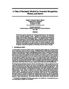
paths before testing the procedure on a set of nonlinear degradation data. For the simulation experiment, sample paths were generated via a known environment process with K distinct states and known degradation rates {r(1), r(2), . . . , r(K)}. Initially, we fix K = 3. Five hundred degradation sample paths, similar to the five shown in Figure 1, were generated for the experiment. PLEASE INSERT FIGURE 1 ABOUT HERE

Setting t0 ≡ 0, we observe the level of degradation at M equally spaced points in time such that tM = 20. That is, the degradation process is observed up to time 20. Figure 2 depicts a sample of observations (M = 10) obtained from the five degradation sample paths of Figure 1 that were used to approximate a piecewise, linear degradation sample path by the procedure of section 4. PLEASE INSERT FIGURE 2 ABOUT HERE

Next, we utilize the approximation to obtain the full and residual lifetime distributions. In each case, we observe the system up to time tM = 20 except that we vary the inter-observation time. In particular, we consider M = 20, 100, and 200 observations on [0, 20], respectively. The assumed unit failure threshold was fixed at x = 152.6 units. The same 500 simulated degradation sample paths were used for each value of M to estimate a new generator matrix and new degradation rates at times 4.0, 8.0, and 12.0, respectively. As before, we compare the estimated versus “true” full lifetime cdfs via the Cram´ervon Mises goodness-of-fit test. Additionally, we compare the estimated versus true residual lifetime distribution. It should be noted that, in order to test the null hypothesis, we use the ˆ t|ξ0 )). The summarized results of Table 2 cdf of the residual lifetime distribution (1 − S(x, 16

indicate that none of the tests are significant at the 0.05 level; thus, we are able to adequately estimate the full and residual lifetime distributions for these simulated degradation paths. PLEASE INSERT TABLE 2 ABOUT HERE

ˆ we simuTo illustrate our method for selecting an appropriate number of states (K), lated multiple degradation sample paths of environment processes having five and ten states, respectively. The F -ratios for each case are displayed in Table 3. Applying the first local ˆ = 4 for the five-state environment and K ˆ = 8 for the maximum rule, the F -ratios suggest K ten-state environment.

PLEASE INSERT TABLE 3 ABOUT HERE

ˆ and K ˆ +1 Consequently, we compared the full and residual lifetime distributions using K states in each scenario. Table 4 indicates that we fail to reject the null hypotheses that the full and residual lifetime distributions are equivalent at the 0.05 level.

PLEASE INSERT TABLE 4 ABOUT HERE

Finally, we illustrate Model II using real degradation data which correspond to the propagation of a fatigue crack in metallic materials. The data were originally analyzed by Virkler, et al. [21] who measured crack length propagation in 68 test specimens of 2024-T3 aluminum alloy. The crack length of each sample was measured over time (in number of load cycles). Figure 3 depicts a representative sample of five degradation paths from the original data set.

PLEASE INSERT FIGURE 3 ABOUT HERE 17

For a more thorough treatment of fatigue crack dynamics, the reader is referred to the paper by Ray and Tangirala [19] and references contained therein. To illustrate our procedure, let X(t) denote the length of the crack at time t and assume the rate at which the crack grows is subject to its random environment (applied stress, ambient conditions, and other factors). It is assumed that these environmental factors can be characterized by {Z(t) : t ≥ 0}, a temporally homogeneous (time-stationary) Markov process on a finite-state sample space. Though the underlying data may, in fact, exhibit nonstationary behavior, we shall observe all 68 sample paths to estimate the generator matrix (Q) for the Z process. In the experiment that follows, the component is said to fail whenever the crack length first exceeds a critical value of x = 45mm. We estimate the off-diagonal generator matrix values by q(i, j) ≈ qˆ(68) =

N (68) (i, j) H (68) (i)

(32)

as defined in Equation (20). It should be noted, however, that the empirical cumulative probabilities for the data were computed with a sample of only 68 observations. Nevertheless, we take this empirical distribution to be the “true” distribution. ˆ was applied to the data by observing 55%, 77%, and The F -ratio test for selecting K 91% of the lifetime, respectively. We select two clusters at 55% of the lifetime, nine clusters at 77% of the lifetime (due to the sharp increase), and twelve clusters at 91% of the lifetime as seen in Table 5.

PLEASE INSERT TABLE 5 ABOUT HERE

ˆ = Estimates of the generator matrix and degradation rates were constructed for K 2, 3, 4, 9, and 12 when observing up to 91% of the lifetime of each specimen. The resulting cdfs (full and residual lifetime) for each case were compared to the empirical distribution at a fixed number of points (m = 65) using the Cram´er-von Mises test. The results of the numerical tests are summarized in Table 6.

18

PLEASE INSERT TABLE 6 ABOUT HERE

ˆ = 2, 3, and 4, we The results for the full lifetime distributions suggest that for K fail to reject the null hypothesis that the distributions are equal. For the residual lifetime ˆ = 3 and 4, we fail to reject the null hypothesis that the distributions distributions with K ˆ = 12. However, using an are equal. The F -ratio test of Table 5 indicates an estimate of K estimated 12-state generator matrix, the resulting full and residual lifetime cdfs fail to pass the goodness-of-fit tests. Although it is apparent that there may exist greater than three or four environmental states, we surmise that the 12-state estimate is poor for a few reasons. First, to adequately estimate a 12-state generator matrix, a fairly large number of environmental transitions must occur during a finite observation period. It is obvious, by inspection of Figure 3 that few significant transitions take place early on. Second, it is likely that transitions occur primarily between a subset of the overall environment sample space at different times. That is, some state transitions appear to dominate early in the specimen lifetimes while others dominate as the specimens age (i.e., as the crack grows). Consequently, we surmise that an age- or degradation-state dependent model may be more appropriate for this data set, as it appears to violate the time-stationarity assumptions of our model. However, it is important to note that the estimation procedure indicated that only a few states could be used within our framework to provide adequate cumulative probability estimates. We surmise that there may exist a minimal representation for the underlying process that includes only the “most important” states. In the current framework, our model does not dynamically dictate which states are most important. Though the distribution results were comparatively disappointing for the empirical data, we conducted an experiment to compare the actual mean lifetime and mean residual lifetime with the results of our models for various failure threshold levels. We computed the mean residual lifetimes by conditioning on the event that a specimen survives beyond the

19

observed, unconditional mean lifetime. For each threshold value, a new generator matrix and degradation rates were estimated using K = 3 environmental states. The mean lifetimes over the 68 degradation paths were compared to those computed by Equation (14). The mean residual lifetimes were computed by Equation (15). The initial measured crack length was approximately 9.0 mm (i.e., X(0) ≈ 9.00 mm). Table 7 summarizes the results of this experiment.

PLEASE INSERT TABLE 7 ABOUT HERE

The results of this experiment indicate that the procedure adequately estimates the mean lifetimes and the mean residual lifetimes. Though not as informative as the residual life distribution, the lower moment approximations may be useful for constructing surrogate parametric distributions.

6

Conclusions In this paper, we have presented a novel approach for the estimation of full and

residual lifetime distributions (and moments) for single-unit systems subject to a Markov environment. The approach provides a necessary first step toward a formal, analytical technique for remaining lifetime prognosis via real degradation measures. Knowledge of the residual lifetime distribution is especially useful for prescribing policies that may reduce the risk of catastrophic failures while eliminating superfluous preventive maintenance activities. Our approach is novel in that we combine analytical stochastic modelling techniques with real sensor data in two distinct cases. First, we considered the case when the sensor data provides real-time information regarding the current state of the environment in which the single-unit system resides. Second, we considered the case in which the sensors provide the current level of degradation of the component. In the first case, our numerical results show great promise for a fully-automated technique for the estimation of lifetime distributions 20

under our problem assumptions. In the second case, we demonstrated that our technique could be used to compute the distributions given nothing more than degradation measures (assumed to be perfectly observable). Though our procedure for estimating residual lifetime distributions performed only moderately well on the empirical data of Virkler, et al. [21], the comparison of mean residual lifetimes is very promising. The techniques presented in this research have raised a few important questions that require further study. First, it may be possible that the time between environment transitions is distinctly non-exponential. In such case, the engineer should resort to phase-type approximations for the state holding time distributions as outlined by Altiok [4]. This approach has the benefit of retaining the Markov property of the environmental process so that the main results of this paper (i.e., Equations (5) and (6)) may still be applied. The disadvantage of this approach is that it requires an expansion of the environment state space. Second, there is the issue of non-stationarity of the environment process. It will be instructive to consider the problem of estimating the parameters of an age-dependent environment process model. Due to extensive data requirements, it appears that this extension may only be feasible if the failure dynamics of the material under consideration are known. Finally, in order to facilitate a fully-automated prognostic system, it will be necessary to develop more robust techniques for evaluating the degradation rates. Such techniques may need to account explicitly for the effects of external covariates as noted in [17].

Acknowledgements: The authors acknowledge, with gratitude, the helpful comments of three anonymous referees and the Associate Editor. This research was supported by the Air Force Office of Scientific Research under agreement QAF185045200004.

References [1] Abate, J. and Whitt, W. (1995) Numerical inversion of Laplace transforms of probability distributions. ORSA Journal on Computing 7, 36-43.

21

[2] Abate, J., Choudhury, G., and Whitt, W. (1998) Numerical inversion of multidimensional Laplace transforms by the Laguerre method, Performance Evaluation 31, 229243. [3] Abdel-Hameed, M. (1984) Life distribution properties of devices subject to L´evy wear process, Mathematics of Operations Research 9, 606-614. [4] Altiok, T. (1985). On the phase-type approximations of general distributions, IIE Transactions 17 (2), 110-116. [5] Basawa, I.V. and Rao, P. (1980) Statistical Inference for Stochastic Processes, John Wiley and Sons, New York. [6] Bogdanoff J.L. and F. Kozin (1985), Probabilistic Models of Cumulative Damage, John Wiley and Sons, New York. [7] Calinski, R.B. and J. Harabasz (1974), A dendrite method for cluster analysis, Communications in Statistics, 3, 1-27. ¸ inlar (1977) Shock and wear models and Markov additive processes, In The Theory [8] E. C and Applications of Reliability (I.N. Shimi and C.P. Tsokos, eds.), Academic, 193-214. [9] Esary, J.D., Marshall, A.W., and Proschan, F. (1973) Shock models and wear processes, Annals of Probability 1, 627-649. [10] Fraley, C. and A Raftery (1998), How many clusters? Which clustering method? Answers via model-based cluster analysis, The Computer Journal, 41, (8), 578-588. [11] Gertsbakh, I.B. and Kordonsky, K.B. (1969) Models of Failure, Springer-Verlag, New York. [12] Gillen, K.T. and Celina, M. (2001) The wear-out approach for predicting the remaining lifetime of materials, Polymer Degradation and Stability, 71, 15-30.

22

[13] Kharoufeh, J.P. (2003) Explicit results for wear processes in a Markovian environment, Operations Research Letters, 31 (3), 237-244. [14] Lee, M.T., DeGruttola, V., and Schoenfeld, D. (2000) A model for markers and latent health status, Journal of the Royal Statistical Society B, 62 (4), 747-762. [15] Lu, C.J. and Meeker, W.Q. (1993) Using degradation measures to estimate a time-tofailure distribution, Technometrics, 35 (2), 161-174. [16] Meeker, W.Q. and Escobar, L.A. (1998) Statistical Methods for Reliability Data, John Wiley and Sons, Inc., New York. [17] Meeker, W.Q., Escobar, L.A., and Chan, V. (2002) Using accelerated tests to predict service life in highly variable environments, in Service Life Prediction: Methodologies and Metrologies, edited by Bauer, D.R. and Martin, J.W., American Chemical Society, Washington, D.C. [18] Moorthy, M.V. (1995) Numerical inversion of two-dimensional Laplace transformsFourier series representation, Applied Numerical Mathematics 17, 119-127. [19] Ray, A. and Tangirala, S. (1997) A nonlinear stochastic model of fatigue crack dynamics, Probabilistic Engineering Mechanics 12, 33-40. [20] Singpurwalla, N.D. (1995) Survival in dynamic environments, Statistical Science 10, 86-103. [21] Virkler, D.A., Hillberry, B.M., and Goel, P.K. (1979) The statistical nature of fatigue crack propagation, ASME Journal of Engineering Materials and Technology, 101 (2), 148-153. [22] Whitmore, G.A., Crowder, M.J., and Lawless, J.F. (1998) Failure inference from a marker process based on a bivariate Wiener process, Lifetime Data Analysis, 4, 229251. 23

Tables and Figures 180

160

Cumulative Degradation

140

120

100

80

60

40

20

0

0

2

4

6

8

10 Time

12

14

16

18

20

Figure 1: A sample of five linear degradation paths.

180

160

Cumulative Degradation

140

120

100

80

60

40

20

0

0

2

4

6

8

10 Time

12

14

16

18

20

Figure 2: Piecewise linear approximation of degradation paths.

24

45

40

Crack Length (mm)

35

30

25

20

15

10

5

0

0

0.5

1

1.5

2

2.5

3

5

Load Cycles (X10 )

Figure 3: The propagation of fatigue crack length for five test specimens. Table 1: Cram´er-von Mises test statistics for Model I experiments (κ∗ =0.461, α = 0.05). Distribution

Run Length

T T T T ˆ 1 − S(x, t|ξ0 ) T (m=50) T Fˆ (x, t) (m=48)

= 100 = 500 = 5000 = 100 = 500 = 5000

K=2

K=5

K = 10

7.013E-03 1.649E-03 9.941E-05 5.511E-03 1.223E-03 5.544E-05

4.233E-02 7.895E-03 9.019E-05 3.821E-02 6.553E-03 8.092E-05

9.477E-03 2.130E-03 1.986E-06 7.455E-03 2.113E-03 2.576E-06

25

Table 2: Cram´er-von Mises test statistics for simulated data (κ∗ = 0.461 at α = 0.05). Fˆ (x, t)

ξ0

ˆ t|ξ0 ) 1 − S(x,

M

Interval

20

[0.0,4.0] 0.0157 4.0 [0.0,8.0] 0.0210 8.0 [0.0,12.0] 0.0247 12.0

0.0189 0.1213 0.1633

100 [0.0,4.0] 0.0095 4.0 [0.0,8.0] 0.0088 8.0 [0.0,12.0] 0.0087 12.0

0.0197 0.0476 0.0639

200 [0.0,4.0] 0.0053 4.0 [0.0,8.0] 0.0051 8.0 [0.0,12.0] 0.0052 12.0

0.0149 0.0336 0.0266

Table 3: F -ratio values for five- and ten-state environments (×105 ). K

Five-state

Ten-state

2 3 4 5 6 7 8 9 10 11 12 13 14 15

1.654973 3.090848 4.067369 3.820857 3.249939 6.678639 7.278563 10.76289 7.383198 5.876550 9.920737 8.558721 15.161074 12.455254

0.285050 0.400770 0.421102 0.660245 0.698204 0.955170 1.144632 1.047932 0.697347 1.306396 1.805007 0.857228 0.858865 1.386817

ˆ states (κ∗ = 0.461, α = 0.05, m = 100). Table 4: Cram´er-von Mises test statistics with K K

ˆ K

5 5 10 10

4 5 8 9

Fˆ (x, t)

ξ0

2.3056E-02 17.5311 3.2317E-02 17.5311 3.5704E-02 13.4249 3.5397E-02 13.4249

26

ˆ t|ξ0 ) 1 − S(x,

1.0179E-01 1.0733E-01 1.6783E-01 1.4709E-01

Table 5: F -ratio comparison (×104 ).

K

2 3 4 5 6 7 8 9 10 11 12 13 14 15

Percentage of Lifetime 55% 77% 91%

0.845912 0.770946 0.700849 0.637918 1.789474 1.984733 2.230180 2.570793 2.785035 3.017830 2.993362 3.714449 4.167025 4.292031

1.716694 2.045060 2.267842 2.412888 2.506080 2.627177 2.658314 2.669967 4.566412 4.974103 5.272737 5.683212 5.850034 6.608150

1.934667 2.448228 2.866000 3.248069 3.620849 3.934574 4.208318 4.374201 4.448147 4.744162 4.830633 4.796518 4.800008 4.745232

Table 6: Cram´er-von Mises test statistic (κ∗ = 0.461 at α = 0.05, m = 65). ˆ K

Fˆ (x, t)

ξ0

ˆ t|ξ0 ) 1 − S(x,

2 3 4 9 12

1.398488E-01 8.671149E-02 4.525246E-01 7.657227E-01 8.723972E-01

2.534 2.534 2.534 2.534 2.534

6.124815E-01 1.395285E-01 4.383202E-01 2.235864E-00 1.667689E-00

Table 7: Mean full and residual lifetimes (×105 load cycles), ξ0 = actual m(1) (x). m(1) (x) x (mm)

10 15 20 25 30 35 41

Actual

m(1) (x|ξ0 )

Model

0.318574 0.325974 1.183405 1.150109 1.638693 1.530864 1.938014 1.800568 2.158575 2.021006 2.326253 2.116553 2.464467 2.298747

27

Actual

Model

0.349943 1.268688 1.738733 2.042441 2.286812 2.458462 2.611653

0.347018 1.293640 1.771963 2.113597 2.368369 2.508772 2.633815